Why symmetric positive-(semi)definite matrices matter

mathematical statistics
Symmetric positive-(semi)definite matrices are fundamental objects in statistics, optimization, and machine learning. Their unique mathematical properties make them indispensable for various statistical applications, from basic covariance estimation to advanced machine learning algorithms.
Author

Yupng L.

Published

November 23, 2025

Introduction

Symmetric positive-(semi)definite matrices are fundamental objects in statistics, optimization, and machine learning. Their unique mathematical properties make them indispensable for various statistical applications, from basic covariance estimation to advanced machine learning algorithms.

Mathematical Foundation

Definition

A symmetric matrix (A symmetric matrix is a square matrix that is equal to its transpose, i.e., A = Aᵀ) \(\mathbf{A} \in \mathbb{R}^{n \times n}\) is:

  • Positive definite if \(\mathbf{x}^T\mathbf{A}\mathbf{x} > 0\) for all \(\mathbf{x} \neq 0\)
  • Positive semi-definite if \(\mathbf{x}^T\mathbf{A}\mathbf{x} \geq 0\) for all \(\mathbf{x}\)

Key Properties

Property Positive definite (PD) Positive semi-definite (PSD)
Quadratic form xᵀAx > 0 ∀ x ≠ 0 xᵀAx ≥ 0 ∀ x
Eigenvalues all > 0 all ≥ 0
Invertibility always invertible may be singular (a square matrix that is not invertible, meaning its determinant is zero and its rank is less than its dimension)
Determinant > 0 ≥ 0
Cholesky decomposition exists (A = LLᵀ) exists only if singularities are handled (e.g., pivoted Cholesky)
Rank full rank can be rank-deficient
Energy interpretation strictly positive energy non-negative energy
Convexity strictly convex quadratic convex (but not necessarily strict)
Statistical role full-rank covariance general covariance (allows perfect collinearity)

positive-definite (PD) ⇔ all eigenvalues > 0

positive-semidefinite (PSD) ⇔ all eigenvalues ≥ 0 (within numeric tolerance)

# Create a positive definite matrix
A <- matrix(c(4, 1, 1, 3), nrow = 2)
colnames(A) <- rownames(A) <- c("X1", "X2")

# Check properties
cat("Matrix A:\n")
Matrix A:
print(A)
   X1 X2
X1  4  1
X2  1  3
cat("\nIs symmetric:", isSymmetric(A))

Is symmetric: TRUE
cat("\nEigenvalues:", eigen(A)$values)

Eigenvalues: 4.618034 2.381966
cat("\nDeterminant:", det(A))

Determinant: 11
cat("\nAll eigenvalues positive:", all(eigen(A)$values > 0))

All eigenvalues positive: TRUE

Equivalence Relations

The following statements are equivalent for a symmetric matrix \(\mathbf{A}\):

  • \(\mathbf{A}\) is positive definite
  • All eigenvalues are positive
  • \(\mathbf{A}\) can be factored as \(\mathbf{A} = \mathbf{L}\mathbf{L}^T\) (Cholesky decomposition)
  • All leading principal minors have positive determinants
  • \(\mathbf{A}\) is invertible with positive definite inverse
# Cholesky decomposition
L <- t(chol(A))
cat("Cholesky factor L:\n")
Cholesky factor L:
cat(L)
2 0.5 0 1.658312
cat("\nReconstruction check (LL'):\n")

Reconstruction check (LL'):
cat(L %*% t(L))
4 1 1 3

Statistical Applications

1. Covariance Matrices

Covariance matrices must be symmetric positive semi-definite by construction. This ensures that:

  • Variances are non-negative: \(\text{Var}(X) = \sigma_{ii} \geq 0\)
  • The Cauchy-Schwarz inequality holds: \(|\sigma_{ij}| \leq \sqrt{\sigma_{ii}\sigma_{jj}}\)
  • Linear combinations have non-negative variance: \(\text{Var}(\mathbf{a}^T\mathbf{X}) = \mathbf{a}^T\boldsymbol{\Sigma}\mathbf{a} \geq 0\)
# Generate multivariate normal data
n <- 1000
p <- 3
Sigma <- matrix(c(1, 0.5, 0.3,
                  0.5, 1, 0.2, 
                  0.3, 0.2, 1), nrow = p)
colnames(Sigma) <- rownames(Sigma) <- c("Var1", "Var2", "Var3")

# Generate data
library(MASS)
X <- mvrnorm(n, mu = rep(0, p), Sigma = Sigma)

# Sample covariance
cov_sample <- cov(X)
cat("Sample covariance matrix:\n")
Sample covariance matrix:
print(round(cov_sample, 3))
      Var1  Var2  Var3
Var1 0.990 0.492 0.323
Var2 0.492 1.012 0.212
Var3 0.323 0.212 0.976
# Check properties
cat("\nIs symmetric:", isSymmetric(cov_sample))

Is symmetric: TRUE
cat("\nEigenvalues:", round(eigen(cov_sample)$values, 3))

Eigenvalues: 1.693 0.795 0.489
cat("\nPositive semidefinite:", all(eigen(cov_sample)$values >= -1e-10))

Positive semidefinite: TRUE

2. Multivariate Normal Distribution

The probability density function requires a positive definite covariance matrix:

\[f(\mathbf{x}) = \frac{1}{(2\pi)^{p/2}|\boldsymbol{\Sigma}|^{1/2}}\exp\left(-\frac{1}{2}(\mathbf{x}-\boldsymbol{\mu})^T\boldsymbol{\Sigma}^{-1}(\mathbf{x}-\boldsymbol{\mu})\right)\]

# Log-likelihood function
log_lik_mvnormal <- function(x, mu, sigma) {
  p <- length(mu)
  det_sigma <- det(sigma)
  inv_sigma <- solve(sigma)
  
  -0.5 * (p * log(2*pi) + log(det_sigma) + t(x - mu) %*% inv_sigma %*% (x - mu))
}

# Test with our data
x_test <- X[1,]
mu_hat <- colMeans(X)
log_lik_mvnormal(x_test, mu_hat, cov_sample)
          [,1]
[1,] -3.687412

To summarize 1 and 2 above: Why Covariance Matrices Must Be PSD??

For any random vector X with covariance matrix Σ, consider a linear combination:

\[ Y = \mathbf{a}^\top \mathbf{X} = a_1 X_1 + a_2 X_2 + \cdots + a_n X_n \]

The variance of \(Y\) is:

\[ \text{Var}(Y) = \text{Var}(\mathbf{a}^\top \mathbf{X}) = \mathbf{a}^\top \boldsymbol{\Sigma} \mathbf{a} \]

Since variance can never be negative:

\[ \mathbf{a}^\top \boldsymbol{\Sigma} \mathbf{a} \geq 0 \quad \text{for all } \mathbf{a} \]

This is exactly the definition of positive semi-definite.

# Any linear combination of random variables has non-negative variance
set.seed(42)
X <- MASS::mvrnorm(1000, mu = c(0, 0), Sigma = matrix(c(1, 0.5, 0.5, 1), 2))
Sigma <- cov(X)

# Pick any weights
a <- c(3, -2)

# Quadratic form = variance of linear combination
quadratic_form <- t(a) %*% Sigma %*% a
actual_variance <- var(X %*% a)

cat("a'Σa =", round(quadratic_form, 4), "\n")
a'Σa = 6.788 
cat("Var(a'X) =", round(actual_variance, 4), "\n")
Var(a'X) = 6.788 
cat("Both non-negative? ", quadratic_form >= 0, "\n")
Both non-negative?  TRUE 

When Is It PD vs Only PSD?

Condition Result
Variables are linearly independent Positive Definite (all λ > 0)
Some variable is a linear combination of others Only PSD (some λ = 0)
# PSD but not PD: X3 = X1 + X2 (perfect linear dependence)
X1 <- rnorm(100)
X2 <- rnorm(100)
X3 <- X1 + X2  # Dependent!

Sigma_singular <- cov(cbind(X1, X2, X3))
eigen(Sigma_singular)$values  # One eigenvalue ≈ 0
[1] 3.194783e+00 1.010505e+00 3.108624e-15

3. Principal Component Analysis (PCA)

PCA requires the covariance matrix to be positive semi-definite to ensure that: - Principal components correspond to directions of maximum variance - Eigenvalues represent explained variances: \(\lambda_i \geq 0\)

# PCA via eigen decomposition
eig_result <- eigen(cov_sample)

# Principal components
PC1 <- eig_result$vectors[,1]
PC2 <- eig_result$vectors[,2]

cat("First principal component:", round(PC1, 3))
First principal component: -0.641 -0.608 -0.468
cat("\nExplained variance (first two):", round(eig_result$values[1:2]/sum(eig_result$values)*100, 1), "%")

Explained variance (first two): 56.9 26.7 %

Optimization Applications

1. Convex Optimization

Positive definite matrices ensure convexity in quadratic optimization:

\[\min_{\mathbf{x}} \mathbf{x}^T\mathbf{A}\mathbf{x} + \mathbf{b}^T\mathbf{x} + c\]

The Hessian matrix \(\nabla^2 f(\mathbf{x}) = 2\mathbf{A}\) must be positive definite for a unique global minimum.

2. Newton’s Method

The Hessian matrix in Newton’s method should be positive definite near the minimum for convergence:

\[\mathbf{x}_{k+1} = \mathbf{x}_k - [\nabla^2 f(\mathbf{x}_k)]^{-1}\nabla f(\mathbf{x}_k)\]

# Newton's method for optimization
newton_optimization <- function(x_init, max_iter = 10) {
  x <- x_init
  
  for(i in 1:max_iter) {
    # Gradient of f(x) = x'Ax + b'x + c
    grad <- 2 * A %*% x + c(1, 1)
    
    # Hessian = 2A (positive definite)
    hessian <- 2 * A
    
    # Newton step
    x_new <- x - solve(hessian) %*% grad
    
    cat(sprintf("Iteration %d: x = [%.4f, %.4f], f(x) = %.4f\n", 
                i, x_new[1], x_new[2], 
                as.numeric(t(x_new) %*% A %*% x_new + c(1,1) %*% x_new)))
    
    if(norm(x_new - x, "F") < 1e-6) break
    x <- x_new
  }
  return(x)
}

# Run optimization
result <- newton_optimization(c(1, 1))
Iteration 1: x = [-0.0909, -0.1364], f(x) = -0.1136
Iteration 2: x = [-0.0909, -0.1364], f(x) = -0.1136

Machine Learning Applications

1. Gaussian Processes

Covariance functions (kernels) must produce positive definite matrices:

\[K(\mathbf{x}, \mathbf{x}') = \sigma^2 \exp\left(-\frac{\|\mathbf{x} - \mathbf{x}'\|^2}{2\ell^2}\right)\]

# RBF kernel function
rbf_kernel <- function(X1, X2, length_scale = 1, sigma_f = 1) {
  dist_matrix <- outer(X1, X2, function(x, y) (x - y)^2)
  sigma_f^2 * exp(-0.5 * dist_matrix / length_scale^2)
}

# Generate kernel matrix
x_points <- seq(-3, 3, length.out = 10)
K <- rbf_kernel(x_points, x_points)

cat("Kernel matrix properties:")
Kernel matrix properties:
cat("\nSymmetric:", isSymmetric(K))

Symmetric: TRUE
cat("\nEigenvalues > 0:", all(eigen(K)$values > 1e-10))

Eigenvalues > 0: TRUE

2. Support Vector Machines

Kernel matrices in SVMs must be positive semi-definite (Mercer’s theorem) for the optimization problem to be convex:

\[K_{ij} = \langle \phi(\mathbf{x}_i), \phi(\mathbf{x}_j) \rangle\]

Numerical Stability and Computational Efficiency

1. Cholesky Decomposition

For positive definite matrices, Cholesky decomposition is twice as efficient as LU decomposition:

\[\mathbf{A} = \mathbf{L}\mathbf{L}^T\]

# Compare decomposition methods
n <- 500
A_large <- Matrix::nearPD(matrix(rnorm(n^2), n, n))$mat

# Cholesky decomposition timing
system.time({
  L <- chol(A_large)
})
   user  system elapsed 
  0.017   0.000   0.018 
# LU decomposition would be slower (commented out for speed)
# system.time({
#   lu_result <- lu(A_large)
# })

2. Matrix Square Root

Positive definite matrices have unique symmetric positive definite square roots:

\[\mathbf{A}^{1/2} = \mathbf{Q}\boldsymbol{\Lambda}^{1/2}\mathbf{Q}^T\]

where \(\mathbf{A} = \mathbf{Q}\boldsymbol{\Lambda}\mathbf{Q}^T\) is the eigen-decomposition.

# Matrix square root via eigendecomposition
sqrt_matrix <- function(A) {
  eig <- eigen(A)
  eig$vectors %*% diag(sqrt(eig$values)) %*% t(eig$vectors)
}

A_sqrt <- sqrt_matrix(A)
cat("A^(1/2):\n")
A^(1/2):
print(round(A_sqrt, 3))
      [,1]  [,2]
[1,] 1.982 0.271
[2,] 0.271 1.711
cat("\nVerification: A^(1/2) * A^(1/2) = A\n")

Verification: A^(1/2) * A^(1/2) = A
print(round(A_sqrt %*% A_sqrt, 3))
     [,1] [,2]
[1,]    4    1
[2,]    1    3

Common Issues and Solutions

1. Numerical Instability

Sample covariance matrices may lose positive definiteness due to rounding errors:

# Add small regularization
regularize_matrix <- function(A, epsilon = 1e-6) {
  A + epsilon * diag(nrow(A))
}

# Create nearly singular matrix
A_near <- matrix(c(1, 1, 1, 1.0001), nrow = 2)
cat("Original eigenvalues:", eigen(A_near)$values)
Original eigenvalues: 2.00005 4.999875e-05
A_regularized <- regularize_matrix(A_near)
cat("\nRegularized eigenvalues:", eigen(A_regularized)$values)

Regularized eigenvalues: 2.000051 5.099875e-05

2. High-Dimensional Data

When \(p > n\), sample covariance matrices are singular. Solutions include:

  • Shrinkage estimation: \(\hat{\boldsymbol{\Sigma}} = \alpha\mathbf{S} + (1-\alpha)\mathbf{T}\)
  • Graphical lasso: Sparse precision matrix estimation
  • Factor models: Low-rank plus sparse decomposition

Conclusion

Symmetric positive-(semi)definite matrices are fundamental to statistics because they:

  1. Ensure mathematical validity of covariance and correlation matrices
  2. Enable efficient computation through specialized algorithms (Cholesky, eigen-decomposition)
  3. Guarantee convexity in optimization problems
  4. Provide geometric interpretation through ellipsoids and quadratic forms
  5. Support advanced methods in machine learning and high-dimensional statistics

Their unique properties make them indispensable tools across the statistical sciences, from basic data analysis to cutting-edge machine learning algorithms. Understanding these matrices is crucial for anyone working in statistics, optimization, or machine learning.

Appendix 1 - Eigenvalues

Eigenvalues tell you how much the matrix stretches space along each eigen-direction; big λ = lots of stretch, tiny λ = almost flat, negative λ = flip + stretch.

Summary: Geometric Meaning of Eigenvalues

Concept Geometric Interpretation
Eigenvector Direction that doesn’t rotate under transformation
Eigenvalue Stretching factor along that direction
λ > 1 Stretch (expand)
0 < λ < 1 Shrink (compress)
λ < 0 Flip (reflect) + scale
λ = 0 Collapse (lose dimension)
Complex λ Rotation (no fixed direction)

For Symmetric Matrices (Covariance/Hessian)

Eigenvalue Sign Matrix Type Geometric Shape
All λ > 0 Positive Definite Bowl (ellipsoid)
All λ < 0 Negative Definite Dome (inverted ellipsoid)
Mixed signs Indefinite Saddle
Some λ = 0 Semi-definite Cylinder/flat direction
# =============================================================================
# GEOMETRIC UNDERSTANDING OF EIGENVALUES
# =============================================================================

library(ggplot2)

# -----------------------------------------------------------------------------
# 1. CORE IDEA: EIGENVECTORS ARE DIRECTIONS THAT DON'T ROTATE
# -----------------------------------------------------------------------------

# Matrix A transforms vectors. Most vectors change direction.
# Eigenvectors ONLY get stretched/shrunk, not rotated.
# Eigenvalue = the stretching factor

A <- matrix(c(3, 1, 1, 2), nrow = 2)
eig <- eigen(A)

cat("Matrix A:\n"); print(A)
Matrix A:
     [,1] [,2]
[1,]    3    1
[2,]    1    2
cat("\nEigenvalues:", round(eig$values, 3))

Eigenvalues: 3.618 1.382
cat("\nλ1 =", round(eig$values[1], 3), "→ stretches by factor", round(eig$values[1], 3))

λ1 = 3.618 → stretches by factor 3.618
cat("\nλ2 =", round(eig$values[2], 3), "→ stretches by factor", round(eig$values[2], 3))

λ2 = 1.382 → stretches by factor 1.382
# -----------------------------------------------------------------------------
# 2. VISUALIZE: HOW A MATRIX TRANSFORMS A CIRCLE
# -----------------------------------------------------------------------------

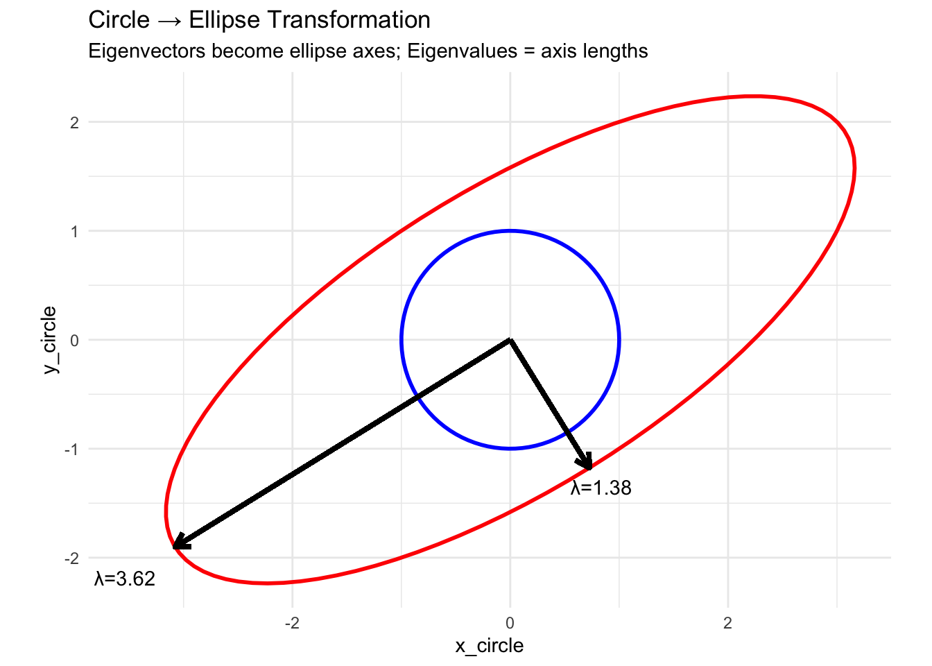
# A circle becomes an ellipse under linear transformation
# Eigenvectors = ellipse axes, Eigenvalues = axis lengths

# Unit circle points
theta <- seq(0, 2*pi, length.out = 100)
circle <- cbind(cos(theta), sin(theta))

# Transform by matrix A
ellipse <- t(A %*% t(circle))

# Eigenvectors (scaled by eigenvalues for visualization)
v1 <- eig$vectors[,1] * eig$values[1]
v2 <- eig$vectors[,2] * eig$values[2]

df <- data.frame(
  x_circle = circle[,1], y_circle = circle[,2],
  x_ellipse = ellipse[,1], y_ellipse = ellipse[,2]
)

ggplot(df) +
  # Original circle
  geom_path(aes(x_circle, y_circle), color = "blue", linewidth = 1) +
  # Transformed ellipse
  geom_path(aes(x_ellipse, y_ellipse), color = "red", linewidth = 1) +
  # Eigenvectors
  geom_segment(aes(x = 0, y = 0, xend = v1[1], yend = v1[2]), 
               arrow = arrow(length = unit(0.3, "cm")), linewidth = 1.2) +
  geom_segment(aes(x = 0, y = 0, xend = v2[1], yend = v2[2]), 
               arrow = arrow(length = unit(0.3, "cm")), linewidth = 1.2) +
  annotate("text", x = v1[1]*1.15, y = v1[2]*1.15, 
           label = paste0("λ=", round(eig$values[1], 2))) +
  annotate("text", x = v2[1]*1.15, y = v2[2]*1.15, 
           label = paste0("λ=", round(eig$values[2], 2))) +
  coord_fixed() +
  labs(title = "Circle → Ellipse Transformation",
       subtitle = "Eigenvectors become ellipse axes; Eigenvalues = axis lengths") +
  theme_minimal()

# -----------------------------------------------------------------------------
# 3. THE EIGENVALUE EQUATION GEOMETRICALLY
# -----------------------------------------------------------------------------

# Av = λv means:
# - Apply matrix A to vector v
# - Result is just v scaled by λ
# - Direction unchanged!

v <- eig$vectors[,1]  # First eigenvector
Av <- A %*% v          # Transform it
lambda_v <- eig$values[1] * v  # Scale by eigenvalue

cat("\n\nEigenvector v:", round(v, 3))


Eigenvector v: -0.851 -0.526
cat("\nA × v =", round(Av, 3))

A × v = -3.078 -1.902
cat("\nλ × v =", round(lambda_v, 3))

λ × v = -3.078 -1.902
cat("\nSame? ", all.equal(as.vector(Av), as.vector(lambda_v)))

Same?  TRUE
# -----------------------------------------------------------------------------
# 4. DIFFERENT EIGENVALUE SCENARIOS
# -----------------------------------------------------------------------------

visualize_transform <- function(A, title) {
  eig <- eigen(A)
  theta <- seq(0, 2*pi, length.out = 100)
  circle <- cbind(cos(theta), sin(theta))
  ellipse <- t(A %*% t(circle))
  
  ggplot() +
    geom_path(aes(circle[,1], circle[,2]), color = "blue", linewidth = 1) +
    geom_path(aes(ellipse[,1], ellipse[,2]), color = "red", linewidth = 1) +
    coord_fixed(xlim = c(-4, 4), ylim = c(-4, 4)) +
    labs(title = title, 
         subtitle = paste("λ =", paste(round(eig$values, 2), collapse = ", "))) +
    theme_minimal()
}

# Case 1: Both eigenvalues positive (ellipse)
A1 <- matrix(c(3, 0.5, 0.5, 1), nrow = 2)

# Case 2: One eigenvalue negative (reflection + stretch)
A2 <- matrix(c(2, 0, 0, -1), nrow = 2)

# Case 3: Complex eigenvalues (rotation)
A3 <- matrix(c(0, -1, 1, 0), nrow = 2)  # 90° rotation

# Case 4: Eigenvalue = 0 (collapse to line)
A4 <- matrix(c(1, 2, 0.5, 1), nrow = 2)

# Print eigenvalue interpretations
scenarios <- list(
  list(A1, "Both λ > 0: Pure stretching"),
  list(A2, "λ1 > 0, λ2 < 0: Stretch + Reflection"),
  list(A3, "Complex λ: Rotation (no real eigenvectors)"),
  list(matrix(c(1, 0, 0, 0), 2), "λ = 0: Collapse dimension")
)

for (s in scenarios) {
  cat("\n", s[[2]], "\n")
  cat("Eigenvalues:", round(eigen(s[[1]])$values, 3), "\n")
}

 Both λ > 0: Pure stretching 
Eigenvalues: 3.118 0.882 

 λ1 > 0, λ2 < 0: Stretch + Reflection 
Eigenvalues: 2 -1 

 Complex λ: Rotation (no real eigenvectors) 
Eigenvalues: 0+1i 0-1i 

 λ = 0: Collapse dimension 
Eigenvalues: 1 0 
# -----------------------------------------------------------------------------
# 5. EIGENVALUES OF SYMMETRIC MATRICES (COVARIANCE)
# -----------------------------------------------------------------------------

# For symmetric matrices (like covariance):
# - Eigenvalues are ALWAYS real
# - Eigenvectors are ALWAYS orthogonal
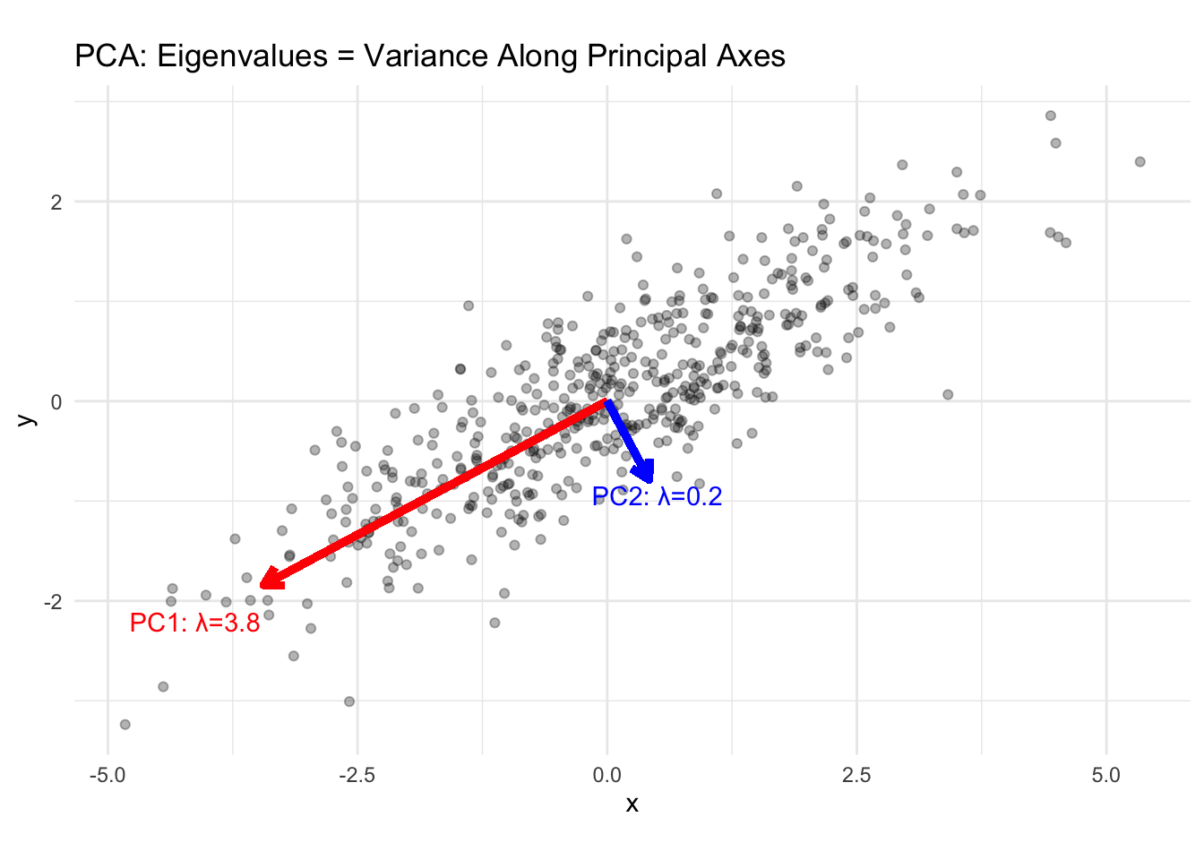
# - Eigenvalues = variance along each principal axis

# Covariance matrix
Sigma <- matrix(c(3, 1.5, 1.5, 1), nrow = 2)
eig_sigma <- eigen(Sigma)

cat("\n\nCovariance Matrix Σ:\n"); print(Sigma)


Covariance Matrix Σ:
     [,1] [,2]
[1,]  3.0  1.5
[2,]  1.5  1.0
cat("\nEigenvalues (variances along PCs):", round(eig_sigma$values, 3))

Eigenvalues (variances along PCs): 3.803 0.197
cat("\nTotal variance:", sum(diag(Sigma)), "=", sum(eig_sigma$values))

Total variance: 4 = 4
# Simulate data
set.seed(42)
data <- MASS::mvrnorm(500, mu = c(0, 0), Sigma = Sigma)

# Plot with eigenvectors
df_data <- data.frame(x = data[,1], y = data[,2])
v1 <- eig_sigma$vectors[,1] * sqrt(eig_sigma$values[1]) * 2
v2 <- eig_sigma$vectors[,2] * sqrt(eig_sigma$values[2]) * 2

ggplot(df_data, aes(x, y)) +
  geom_point(alpha = 0.3) +
  geom_segment(aes(x = 0, y = 0, xend = v1[1], yend = v1[2]), 
               color = "red", linewidth = 1.5,
               arrow = arrow(length = unit(0.3, "cm"))) +
  geom_segment(aes(x = 0, y = 0, xend = v2[1], yend = v2[2]), 
               color = "blue", linewidth = 1.5,
               arrow = arrow(length = unit(0.3, "cm"))) +
  annotate("text", x = v1[1]*1.2, y = v1[2]*1.2, 
           label = paste0("PC1: λ=", round(eig_sigma$values[1], 2)), color = "red") +
  annotate("text", x = v2[1]*1.2, y = v2[2]*1.2, 
           label = paste0("PC2: λ=", round(eig_sigma$values[2], 2)), color = "blue") +
  coord_fixed() +
  labs(title = "PCA: Eigenvalues = Variance Along Principal Axes") +
  theme_minimal()

# -----------------------------------------------------------------------------
# 6. EIGENVALUES AND DEFINITENESS (BACK TO HESSIAN)
# -----------------------------------------------------------------------------

cat("\n\n=== Connection to Optimization ===\n")

=== Connection to Optimization ===
check_definiteness <- function(A) {
  eig <- eigen(A, symmetric = TRUE)$values
  cat("Eigenvalues:", round(eig, 3), "\n")
  
  if (all(eig > 0)) {
    cat("→ All positive → PD → CONVEX (bowl shape)\n")
  } else if (all(eig < 0)) {
    cat("→ All negative → ND → CONCAVE (dome shape)\n") 
  } else if (all(eig >= 0)) {
    cat("→ Non-negative → PSD → Convex (may be flat)\n")
  } else {
    cat("→ Mixed signs → INDEFINITE → SADDLE POINT\n")
  }
}

cat("\nConvex Hessian:\n")

Convex Hessian:
check_definiteness(matrix(c(2, 0.5, 0.5, 3), 2))
Eigenvalues: 3.207 1.793 
→ All positive → PD → CONVEX (bowl shape)
cat("\nConcave Hessian:\n")

Concave Hessian:
check_definiteness(matrix(c(-2, 0.5, 0.5, -3), 2))
Eigenvalues: -1.793 -3.207 
→ All negative → ND → CONCAVE (dome shape)
cat("\nSaddle Point Hessian:\n")

Saddle Point Hessian:
check_definiteness(matrix(c(2, 0, 0, -3), 2))
Eigenvalues: 2 -3 
→ Mixed signs → INDEFINITE → SADDLE POINT

Appendix 2 - Derivation: Var(a’X) = a’Σa

Step 1: Definition of Variance

For any random variable \(Y\):

\[ \text{Var}(Y) = E\left[(Y - E[Y])^2\right] \]

Step 2: Let \(Y = \mathbf{a}^\top \mathbf{X}\)

The expected value of \(Y\) is:

\[ E[Y] = E[\mathbf{a}^\top \mathbf{X}] = \mathbf{a}^\top E[\mathbf{X}] = \mathbf{a}^\top \boldsymbol{\mu} \]

Step 3: Substitute into Variance Formula

\[ \text{Var}(\mathbf{a}^\top \mathbf{X}) = E\left[(\mathbf{a}^\top \mathbf{X} - \mathbf{a}^\top \boldsymbol{\mu})^2\right] \]

Step 4: Factor Out \(\mathbf{a}^\top\)

\[ = E\left[(\mathbf{a}^\top (\mathbf{X} - \boldsymbol{\mu}))^2\right] \]

Step 5: Expand the Square

Since \(\mathbf{a}^\top (\mathbf{X} - \boldsymbol{\mu})\) is a scalar, its square equals:

\[ (\mathbf{a}^\top (\mathbf{X} - \boldsymbol{\mu}))^2 = \mathbf{a}^\top (\mathbf{X} - \boldsymbol{\mu})(\mathbf{X} - \boldsymbol{\mu})^\top \mathbf{a} \]

Step 6: Take Expectation

\[ \text{Var}(\mathbf{a}^\top \mathbf{X}) = E\left[\mathbf{a}^\top (\mathbf{X} - \boldsymbol{\mu})(\mathbf{X} - \boldsymbol{\mu})^\top \mathbf{a}\right] \]

Since \(\mathbf{a}\) is constant:

\[ = \mathbf{a}^\top E\left[(\mathbf{X} - \boldsymbol{\mu})(\mathbf{X} - \boldsymbol{\mu})^\top\right] \mathbf{a} \]

Step 7: Recognize Covariance Matrix

By definition:

\[ \boldsymbol{\Sigma} = E\left[(\mathbf{X} - \boldsymbol{\mu})(\mathbf{X} - \boldsymbol{\mu})^\top\right] \]

Final Result

\[ \boxed{\text{Var}(\mathbf{a}^\top \mathbf{X}) = \mathbf{a}^\top \boldsymbol{\Sigma} \mathbf{a}} \]


Key Trick: Scalar Square as Quadratic Form

The crucial step is recognizing that for a scalar \(s = \mathbf{a}^\top \mathbf{b}\):

\[ s^2 = s \cdot s = (\mathbf{a}^\top \mathbf{b})(\mathbf{b}^\top \mathbf{a}) = \mathbf{a}^\top \mathbf{b} \mathbf{b}^\top \mathbf{a} \]

This converts a squared scalar into a quadratic form.