A Bayesian Single-Arm Design Using PP Monitoring (Replication of Paper from AZ)
Introduction
This document aims to replicate the results from the paper:
Mitchell PD. A Bayesian single-arm design using predictive probability monitoring. Biom Biostat Int J. 2018;7(4):299-309. DOI: 10.15406/bbij.2018.07.00222 link
This design is an additional option for single arm designs where there is a desire to stop early for futility in a flexible way.
With this design, fewer patients will be exposed to ineffective compounds than would be exposed using either a single arm trial with either no or a fixed interim.
As with all designs the operating characteristics should be carefully understood before conducting the corresponding experiment. In the case of compounds that show more activity, more patients will be exposed to the compound in anticipation of progressing into later phase development.
Predictive probability can be used as an effective means to continuously monitor the chance of success in an ongoing single-arm trial.
Study Design
This design is a single arm design in which patients either respond to an experimental treatment or not after being followed for a fixed amount of time. Patients will be enrolled in the trial in four sequential phases. The overall sample will be N=Na+Nb+Nc+Nd patients.
The responses of the individual patients to treatment will be denoted by Yi (i=1 … N). The chance that patient i responds is \(\theta\). The behavior of \(\theta\) is described in the section below on “True Effect Distribution”.
Na patients will be enrolled and evaluated unconditionally based on efficacy response. Once the efficacy response is observed in patient Na, trial monitoring using predictive probability including all Na patients begins.
If predictive probability that the proportion of patients responding is at least \(\tau\) falls below some level \(\phi\) then the trial will be permanently stopped for futility. If the trial is not stopped then the efficacy response for the first patient in Phase b (Patient Na+1) will be observed, predictive probability will then be recalculated for all Na+1 patients and the same criterion will be applied (if predictive probability \(> \phi\) then continue to the next patient. Otherwise, the trial will be stopped.). The observation of efficacy response in each patient enrolled during Phase b followed by the calculation of predictive probability will continue for all patients in this phase for as long as predictive probability remains above \(\phi\).
If the trial continues through all patients planned in Phase b, then following the observation of the response of the next patient (Phase c), an interim analysis with both futility and administrative facets including all patients up through Phase c will be conducted. This interim will include two criteria:
- a ‘stop’ criterion (S) where the trial will stop if the proportion of patients who respond to treatment is equal to or below this level and
- a ‘go’ (G) criterion where other actions associated with more robust efficacy could be taken.
If the trial does not stop, as a result of the interim analysis, then the balance of the planned Nd patients, will be enrolled and a final analysis including all N patients will be conducted.
Temporary stopping is not assumed during the trial. This analysis will be similar to the interim in that the proportion of patients who respond will be evaluated using two criteria (‘STOP’ and ‘GO’).
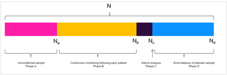
A schema of study design.
Import R packages
# load package
library(ggplot2)
library(dplyr)
library(rtables)
library(knitr)
library(tidyr)
library(gridExtra)
library(reshape)
library(gcookbook)
library(flextable)
library(cowplot)
Functions to be used
Beta prior
The selection of a prior other than one that is non-informative is beyond the scope of this paper, if there is enough information in patients with the disease under study available that information can be used to construct an empirical prior for the true response proportion.
The number of responses in the sample will follow a Binomial distribution with true response parameter \(\theta\). A natural choice for the True Effect distribution of \(\theta\) is Beta with parameters \(\alpha + 1\) and \(\beta + 1\). These can be selected as functions of the mean proportion of responders and an equivalent sample size Morita.
Morita S, Thall PF, Müller P. Determining the Effective Sample Size of a Parametric Prior. Biometrics. 2008;64(2):595–602.
The Nt is the strength of the True Effect distribution in terms of a sample size equivalent which will allow for rational values (ranging from 0, equivalent to a Uniform (0,1) to large values which yield distributions where almost all of the density is within a small neighborhood of the mean).
Prop is the mean of the True Effect distribution. When evaluating the opearting characteristics of the design, Nt should be no more than 10% of the overall sample size. A range of Prop values (selected to cover the parameter space) are used to assess design performance.
###################
## Prior
###################
Beta_ab <- function(Nt, Prop) {
  # Nt  :   Sample size (numeric > 0, REAL)
  # Prop    :   Mean Proportion ( (0,1) )
  if ((Nt >= 0) & ((Prop >= 0) & (Prop <= 1))) {
    alpha <- Nt * Prop
    beta <- Nt * (1-Prop)
    param <- c(alpha, beta)
  }
  else
    param <- NA
  return(param)
}
Predictive power monitoring from a specified start patient until IA
Jennison C, Turnbull BW. Group Sequential Methods Applications to Clinical Trials. USA: Chapman & Hall/CRC Press; 2000.
Predictive power is presented in Jennison & Turnbull and is similar to the expression shown below.
For a single arm trial with \(N\) planned patients and an interim analysis to occur following \(N_{I}\) patients (\(N_{I}\) \(< N\)), where \(n_{I}\) of the \(N_{I}\) patients included in the interim respond and we need to observe \(n_{S}\) (\(n_{S} > n_{I}\)) patients in order to declare the trial a success then the predictive or the chance to observe at least \(n_{S}\) patients out of \(N\) patients (at the end of the trial) is:
\[\sum_{ISS = 0}^{N_{I}}\left\lbrack \Pr(X = ISS \mid \frac{n_{I}}{N_{I}}) \times (1 - \Pr(Y \leq (n_{S} - n_{I} - 1) \mid \theta = \frac{ISS}{N_{I}})) \right\rbrack\]
The important difference is that predictive power implies that the target is a function of a critical value. Predictive probability allows for the selection of a target other than the critical value. The specifics of the application to non-comparative trials with binomial endpoints are described here.
The left hand factor in the expression \(\Pr(X = ISS \mid \frac{n_{I}}{N_{I}})\) being summed above is a vector of probabilities that \(ISS\) responses are observed assuming that the observed response proportion is actually true.
The right hand factor \(1 - \Pr(Y \leq (n_{S} - n_{I} - 1) \mid \theta = \frac{ISS}{N_{I}})\) is the probability that at least the balance of the required responses needed is observed in the remaining patients to be observed in the planned sample.
\(X \sim Bin(N_{I},\frac{ISS}{N_{I}})\) and \(X\) ranges from 0 to \(N_{I}\) and is the possible number of successes observed at an interim with \(N_{I}\) total observations.
\(Y\) is the number of succeses that remain following the interim necessary to achieve the target at the end of the trial.
###################
## Predictive prob
###################

pred_power_bin <- function(N, N_I, ns, ni) {
  # N   :   Total N planned in sample
  # N_I :   N (sample size) at interim
  # ns  :   Number of success needed in total sample
  # ni  :   Number of successes observed at interim

  ISS <- 0:N_I                      #   Interim sample space
  LIK <- dbinom(ISS, N_I, ni / N_I, log = FALSE)    #   Likelihood of interim result given interim observed result

  mid_e <- length(ISS)
  mid <- ISS / N_I

      # Exception when ISS=0
      mid[1] <- ifelse(mid[1] == 0, 0.5 / N_I, ISS / N_I)
      # Exception when ISS=N_I
      mid[mid_e] <- (ISS[mid_e] - 0.5) / N_I

      #Prob of Success
      POS <-
        1 - pbinom((ns - ni) - 1,
                   N - N_I ,
                   mid,
                   lower.tail = TRUE,
                   log.p = FALSE)

      # probability of success at final given interim over all interim results
      assu <- LIK * POS

      return(round(sum(assu), 2))
    }
Main function to perform simulation
Before introducing the simulation function, the strategy of making decisions should be summarized.
A question may be raised firstly: is beta(1,1) using for calculating the posterior probability of response rate when making decisions? Take beta(1,1) as the prior distribution, the posterior distribution for response rate in final analysis is calculated as beta(1+k,1+N-k), where k is the number of responses and N is the total sample size.
For the decision boundaries, for example, can be used to construct rules for advancing compound development.
Decision boundary from literature
For example, 80% confidence that p>LRV might be desired to limit the risk of progressing a compound with relatively little efficacy.
The drug development team will also desire a compound that is commercially viable (p>TV). To avoid terminating such a compound, 10% risk might be chosen.
- Go decision if : PCT20>LRV and PCT90>TV
- Pause if : PCT20<=LRV and PCT90>TV
- Stop if : PCT90<=TV
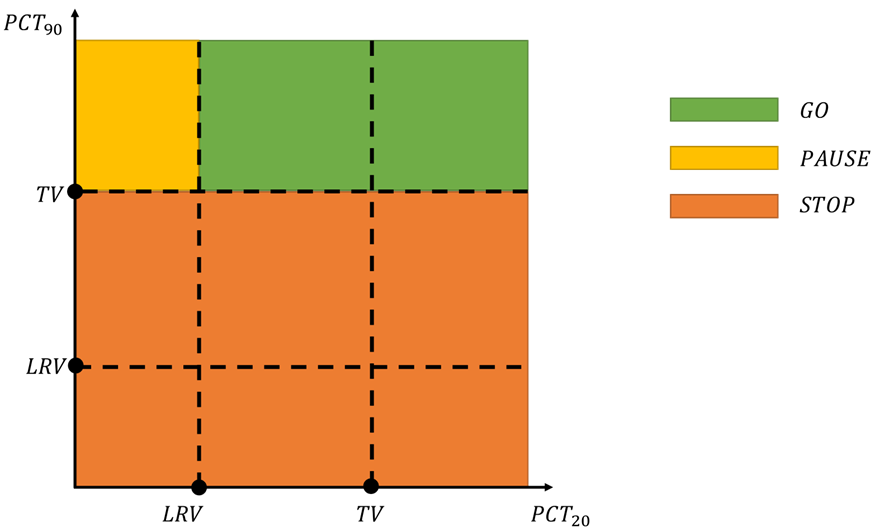
An illustration of decision making
where PCT\(x\) denotes the \(x\)-th percentile of \(\Pr\)(response rate).
The dual criteria can be used to formulate a Go/Pause/Stop decision structure as follows:
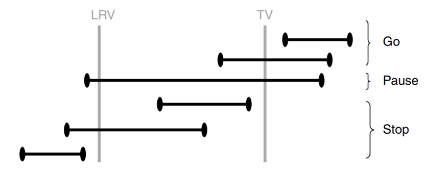
Example of a decision rule based on the dual criteria. The criteria and decisions will vary depending on the target responses that are important for a particular compound and the phase of clinical development.
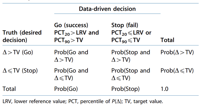
An example of a design performance (trial metrics) summary
Decision boundary described in this paper
The decision criteria used in the design described in this paper are not set directly but are a function of two values selected by the project and are a reflection of the performance necessary to support decisions to go forward in development or to stop development.
These are the target value (TV) and lower reference value (LRV).
In this design:
- A GO decision will be made if
- the posterior probability that the true response proportion is at least LRV is at least DC_LRV.
\[\Pr\lbrack p \geq LRV \mid x\rbrack \geq DC\_ LRV\]
- A STOP decision is made if
- the posterior probability that the true response proportion is at least the TV is no more than AR_TV.
\[\Pr\lbrack p \geq TV \mid x\rbrack \leq AR\_ TV\]
(3)*In cases where both conditions are true (a Go decision and a Stop decision are made simultaneously), a STOP decision is made.
Here the DC_LRV is the desired confidence that the true response proportion is at least as high as the LRV given a GO decision. The AR_TV is the acceptable risk that the true response proportion is at least as high as the TV given a decision to STOP.
###################
## Simulation
###################

trials <- function(Nt,
                   N_i,
                   N_p,
                   true_1,
                   tv,
                   lrv,
                   dc_lrv,
                   ar_tv,
                   Tar, #   Proportion of responders to be observed at final that will lead to a non-stop decision
                   strt, #  Begin predictive power calculation with this observation
                   stop, #  Last patient to monitor via predictive power
                   PPmon ) { #  Minimum predicted power needed to continue arm

  # Sample response rate from prior
  Bpar1 <- Beta_ab(N_p, true_1)
  theta_1 <- rbeta(1, Bpar1[1] + 1, Bpar1[2] + 1)

  # Generate simulated data for total N patients
  arm1 <- rbinom(Nt, 1, theta_1)

  # Take the first N_i data from the complete simulated data arm1 as the data for IA
  int_arm1 <- arm1[1:N_i]

  #########################################################################

  # set data container for storing the results of PP monitoring
  PP1 <- vector(mode = "numeric", length = stop - strt)

  # set data container for storing the number of patients when monitoring PP
  PP1_N <- vector(mode = "numeric", length = stop - strt)

  # set data container for recording the step when monitoring PP
  h <- vector(mode = "numeric", length = stop - strt)

  for (g in 1:(stop - strt)) {
    h[g] <- g
    PP1_N[g] <- strt + (g - 1)
    PP1[g] <-
      pred_power_bin(Nt, strt + (g - 1), round(Nt * Tar, 0), max(sum(int_arm1[1:(strt + (g - 1))])))
  }

  # PP || #pts when doing this PP
  pptab <- data.frame(PP1, PP1_N)

  # Store the results of NOT to continue arm
  ppck1 <- pptab[pptab$PP1 < PPmon, ]

  # exceptions
  ppN1 <- ifelse(length(ppck1$PP1_N) == 0, 0, min(ppck1$PP1_N))

  # records how many patients WIN before futility stopping during PP monitoring
  # a1NPP: the number of patients before NO Continue decision is made
  if (min(pptab$PP1) >= PPmon){
    a1NPP <- N_i
  } else {
    a1NPP <- ppN1
  }

  #########################################################################

  # calculate the REAL number of corresponders among all patients
  sc1 <- sum(arm1)

  # calculate the REAL number of NON-corresponders among all patients
  fa1 <- Nt - sc1

  # calculate the REAL number of corresponders among patients in Interim Analysis
  isc1 <- sum(int_arm1)

  # calculate the REAL number of NON-corresponders among patients in Interim Analysis
  ifa1 <- N_i - isc1

  #########################################################################

  #     Decide

  # For final analysis
  ### 1 for GO, 2 for STOP
  arm1_go <- pbeta(lrv, 1 + sc1, 1 + fa1, lower.tail = FALSE)
  arm1_stop <- pbeta(tv, 1 + sc1, 1 + fa1, lower.tail = FALSE)
  FA_GO_FLAG <- ifelse(arm1_go >= dc_lrv, 1,0)
  FA_STOP_FLAG <- ifelse(arm1_stop <= ar_tv, 2,0)
  arm1_rag <- ifelse(FA_GO_FLAG*FA_STOP_FLAG==0,max(FA_GO_FLAG,FA_STOP_FLAG),2)

  # For interim analysis
  iarm1_go <- pbeta(lrv, 1 + isc1, 1 + ifa1, lower.tail = FALSE)
  iarm1_stop <- pbeta(tv, 1 + isc1, 1 + ifa1, lower.tail = FALSE)
  IA_GO_FLAG <- ifelse(iarm1_go >= dc_lrv, 1,0)
  IA_STOP_FLAG <- ifelse(iarm1_stop <= ar_tv, 2,0)
  iarm1_rag <- ifelse(IA_GO_FLAG*IA_STOP_FLAG==0,max(IA_GO_FLAG,IA_STOP_FLAG),2)

  #########################################################################

  #     Summarize the results

  ## For interim analysis:
  ## if trial early stop since STOP is made in IA, record the sample size for IA
  a1N <-
    ifelse(iarm1_rag == 2, ifelse(a1NPP < N_i, a1NPP, N_i), Nt)
  tot_N <- a1N
  pre_int1 <- ifelse(a1NPP < N_i, "STOP", "GO")
  p <- true_1
  ne <- N_p

  # change flag to char
  FA_FL <- recode(arm1_rag, `2` = "STOP", `1` = "GO")
  IA_FL <- recode(iarm1_rag, `2` = "STOP", `1` = "GO")

  # Package results
  tr <-
    data.frame(
      ne,
      p,
      sc1, # the REAL number of corresponders among all patients
      fa1, # the REAL number of NON-corresponders among all patients
      arm1_go, # boundary for GO at FA
      arm1_stop, # boundary for STOP at FA
      FA_FL, # Decision at FA
      isc1, # the REAL number of corresponders among patients in IA
      ifa1, # the REAL number of NON-corresponders among patients in IA
      iarm1_go, # boundary for GO at IA
      iarm1_stop, # boundary for STOP at IA
      IA_FL, # Decision at IA
      a1NPP, # the number of patients before NO Continue decision is made
      pre_int1, # indicate if trial stops before IA
      a1N, # the sample size when trial stops
      tot_N # the same as a1N
    )

  return(tr)
}
Figure 2
ss <- 50
responders <- seq(0,ss,by=1)
lrv <- 0.3
tv <- 0.5

# function to calculate posterior probability
PostProb <- function(x, boundary,ss){
  return(pbeta(boundary, 1 + x, 1 + ss-x, lower.tail = FALSE))
}

##############
## Figure 2
##############

# create data frame container
PostProbDF1 <-
  data.frame(
    responders = responders,
    goprob = rep(NA, length(responders)),
    stopprob = rep(NA, length(responders))
  )

# retrieve results
for (index in 1:length(responders)){
  PostProbDF1[index,"goprob"] <- PostProb(PostProbDF1[index,"responders"],lrv,ss)
  PostProbDF1[index,"stopprob"] <- PostProb(PostProbDF1[index,"responders"],tv,ss)
}

# reshape data to plot
PostProbDF1_t <- melt(PostProbDF1,id=c("responders"))

# Plot
CritPlot1 <- ggplot(PostProbDF1_t, aes(x=responders, y=value, group=variable)) +
  geom_line(aes(linetype=variable),size=1.2,color="black")+
  geom_hline(yintercept = c(0.1,0.8),linetype=3) +
  geom_point(aes(x=18,y=0.8),colour="black",size=4,shape=18) +
  geom_point(aes(x=20,y=0.1),colour="black",size=4,shape=18) +
  annotate("rect", xmin = 20, xmax = ss, ymin = 0, ymax = 1,alpha = .2,fill = "green") +
  annotate("rect", xmin = 0, xmax = 20, ymin = 0, ymax = 1,alpha = .2,fill = "red") +
  annotate(geom="text", x=4, y=0.75, label="STOP REGION",color="black") +
  annotate(geom="text", x=35, y=0.75, label="GO REGION",color="black") +
  scale_x_discrete(name ="Responders", limits=seq(0,ss,by=5)) +
  scale_y_continuous(name="posterior prob.", limits=c(0, 1))+
  theme_classic()

CritPlot1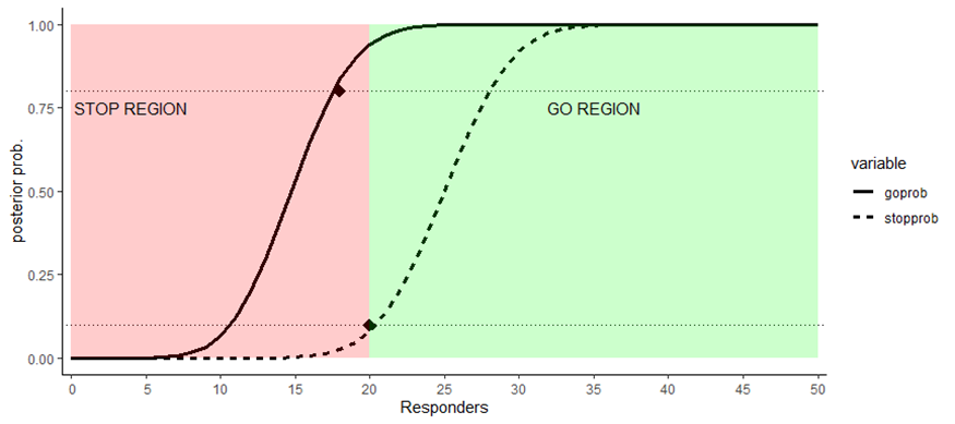
Then we want to find the corresponding number of responders for GO/STOP decision:
# find the number of responders for GO decision
PostProbDF1_t_GO <- PostProbDF1_t %>%
  filter(variable=="goprob" & value>0.8)

min_go_resp <- PostProbDF1_t_GO[1,"responders"]
cat("The minimum responders for GO is: ", min_go_resp, "\n")
## The minimum responders for GO is:  18
# find the number of responders for STOP decision
PostProbDF1_t_STOP <- PostProbDF1_t %>%
  filter(variable=="stopprob" & value<=0.1)

max_stop_resp <- PostProbDF1_t_STOP[length(PostProbDF1_t_STOP$responders),"responders"]
cat("The maximum responders for STOP is: ", max_stop_resp, "\n")
## The maximum responders for STOP is:  20
If the number of responders \(\geq 18\), then a GO decision will be made.
If the number of responders \(\leq 20\), then a STOP decision will be made.
In this case, a STOP decision will be made if the number of responders falls in the interval \(\lbrack 18,20\rbrack\) based on the decision making strategy described in the above section.
Figure 3
##############
## Figure 3
##############

ss <- 30
responders <- seq(0,ss,by=1)

# create data frame container
PostProbDF2 <-
  data.frame(
    responders = responders,
    goprob = rep(NA, length(responders)),
    stopprob = rep(NA, length(responders))
  )

# retrieve results
for (index in 1:length(responders)){
  PostProbDF2[index,"goprob"] <- PostProb(PostProbDF2[index,"responders"],lrv,ss)
  PostProbDF2[index,"stopprob"] <- PostProb(PostProbDF2[index,"responders"],tv,ss)
}

# reshape data to plot
PostProbDF2_t <- melt(PostProbDF2,id=c("responders"))

# Plot
CritPlot2 <- ggplot(PostProbDF2_t, aes(x=responders, y=value, group=variable)) +
  geom_line(aes(linetype=variable),size=1.2,color="black")+
  geom_hline(yintercept = c(0.1,0.8),linetype=3) +
  geom_point(aes(x=11,y=0.8),colour="black",size=4,shape=18) +
  geom_point(aes(x=11,y=0.1),colour="black",size=4,shape=18) +
  annotate("rect", xmin = 11, xmax = ss, ymin = 0, ymax = 1,alpha = .2,fill = "green") +
  annotate("rect", xmin = 0, xmax = 11, ymin = 0, ymax = 1,alpha = .2,fill = "red") +
  annotate(geom="text", x=4, y=0.75, label="STOP REGION",color="black") +
  annotate(geom="text", x=22, y=0.75, label="GO REGION",color="black") +
  scale_x_discrete(name ="Responders", limits=seq(0,ss,by=5))+
  scale_y_continuous(name="posterior prob.", limits=c(0, 1))+
  theme_classic()

CritPlot2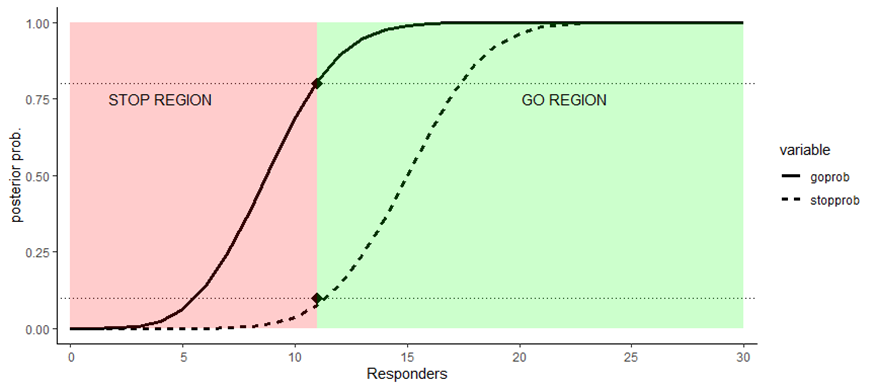
Then we want to find the correponding number of responders for GO/STOP decision:
# find the number of responders for GO decision
PostProbDF2_t_GO <- PostProbDF2_t %>%
  filter(variable=="goprob" & value>0.8)

min_go_resp <- PostProbDF2_t_GO[1,"responders"]
cat("The minimum responders for GO is: ", min_go_resp, "\n")
## The minimum responders for GO is:  11
# find the number of responders for STOP decision
PostProbDF2_t_STOP <- PostProbDF2_t %>%
  filter(variable=="stopprob" & value<=0.1)

max_stop_resp <- PostProbDF1_t_STOP[length(PostProbDF2_t_STOP$responders),"responders"]
cat("The maximum responders for STOP is: ", max_stop_resp, "\n")
## The maximum responders for STOP is:  11
If the number of responders \(\geq 11\), then a GO decision will be made.
If the number of responders \(\leq 11\), then a STOP decision will be made.
In this case, a STOP decision will be made if the number of responders equals to \(11\) based on the decision making strategy described in the above section.
Table 1
# set seed
set.seed(125)

#   Target value
TV <- 0.5

#   Lower reference value
LRV <- 0.3

#   Range of true responses to be explored (combination) in increasing order
True_range <- c(0.8, 0.6, 0.4, 0.2)

#   Strength of prior as a sample size equivalent
PN <- c(0,0.5,1,5,10,20)

#   Planned total sample size
N <- 50

#   Planned interim sample size
Ni <- 30

#   Number of simulated trials
iter <- 4000

#   Minimum predicted power needed to continue arm
MON_stop <- 0.05

#   Proportion of responders to be observed at final that will lead to a non-stop decision
## Target <- 20 / 50
Target <- 0.52

#   Last patient to monitor via predictive power
PP_stop <- 29

#   Begin predictive power calculation with this observation
PP_start <- 12

#   Go: at least 80% chance that the true is greater than the LRV based on the data
DC_LRV <- 0.8

#   Stop: no more than 10% chance that the true is greater than the TV based on the data
AR_TV <- 0.1

# Initiate parameters/data containers to be used in simulations
LenTrueResp <- length(True_range)

SimDataTab1 <-
  data.frame(matrix(NA, length(PN) * length(True_range) * iter, 16)) # create matrix container

a <- 0
row <- 1

if (file.exists("SimDataTab1.RData")) {
  load("SimDataTab1.RData")
} else {
  for (ne in (PN)) {
    for (i in 1:LenTrueResp) {
      # loop through different REAL response rate
      a <- a + 1
      for (z in 1:iter) {
        # loop to generate multiple times of trial
        sim_t <-
          trials(
            N,
            Ni,
            ne,
            True_range[i],
            TV,
            LRV,
            DC_LRV,
            AR_TV,
            Target,
            PP_start,
            PP_stop,
            MON_stop
          )
        SimDataTab1[row, 1:16] <- sim_t[1,]
        row <- row + 1
      }
    }
  }
  colnames(SimDataTab1) <- colnames(sim_t)
  save(SimDataTab1, file = "SimDataTab1.RData")
  load("SimDataTab1.RData")
}

Table1DFMeanSample <- SimDataTab1 %>%
  group_by(ne, p) %>%
  summarise(mean = mean(a1N))

Table1DFProp <- SimDataTab1 %>%
  group_by(ne, p, FA_FL) %>%
  summarise(cnt = n()) %>%
  mutate(freq = round(100*cnt/iter,3)) %>%
  select(-c(cnt)) %>%
  spread(FA_FL, freq) %>%
  arrange(ne,desc(p))

Table1 <- Table1DFMeanSample %>%
  inner_join(Table1DFProp, by = c("ne","p")) %>%
  arrange(ne,desc(p))

flextable(Table1) %>%
FitFlextableToPage()| ne | p | mean | GO | STOP |
|---|---|---|---|---|
| 0.0 | 0.8 | 35.81275 | 59.225 | 40.775 |
| 0.0 | 0.6 | 35.79075 | 59.175 | 40.825 |
| 0.0 | 0.4 | 35.85800 | 58.350 | 41.650 |
| 0.0 | 0.2 | 35.79200 | 58.725 | 41.275 |
| 0.5 | 0.8 | 39.04450 | 67.075 | 32.925 |
| 0.5 | 0.6 | 37.14850 | 62.150 | 37.850 |
| 0.5 | 0.4 | 34.88125 | 55.650 | 44.350 |
| 0.5 | 0.2 | 33.09600 | 50.950 | 49.050 |
| 1.0 | 0.8 | 41.45075 | 73.500 | 26.500 |
| 1.0 | 0.6 | 38.90525 | 66.600 | 33.400 |
| 1.0 | 0.4 | 35.24575 | 56.075 | 43.925 |
| 1.0 | 0.2 | 31.19750 | 45.950 | 54.050 |
| 5.0 | 0.8 | 48.41575 | 94.975 | 5.025 |
| 5.0 | 0.6 | 43.66650 | 79.900 | 20.100 |
| 5.0 | 0.4 | 34.88825 | 54.325 | 45.675 |
| 5.0 | 0.2 | 23.59450 | 23.225 | 76.775 |
| 10.0 | 0.8 | 49.58125 | 98.775 | 1.225 |
| 10.0 | 0.6 | 45.67225 | 86.150 | 13.850 |
| 10.0 | 0.4 | 34.38025 | 49.725 | 50.275 |
| 10.0 | 0.2 | 19.80475 | 12.875 | 87.125 |
| 20.0 | 0.8 | 49.95800 | 99.850 | 0.150 |
| 20.0 | 0.6 | 47.55200 | 91.625 | 8.375 |
| 20.0 | 0.4 | 34.91675 | 50.000 | 50.000 |
| 20.0 | 0.2 | 17.17400 | 5.600 | 94.400 |
Table 2
# set seed
set.seed(125)

#   Proportion of responders to be observed at final that will lead to a non-stop decision
Target <- 0.40

# Initiate parameters/data containers to be used in simulations
SimDataTab2 <-
  data.frame(matrix(NA, length(PN) * length(True_range) * iter, 16)) # create matrix container

a <- 0
row <- 1

if (file.exists("SimDataTab2.RData")) {
  load("SimDataTab2.RData")
} else {
  for (ne in (PN)) {
    for (i in 1:LenTrueResp) {
      # loop through different REAL response rate
      a <- a + 1
      for (z in 1:iter) {
        # loop to generate multiple times of trial
        sim_t <-
          trials(
            N,
            Ni,
            ne,
            True_range[i],
            TV,
            LRV,
            DC_LRV,
            AR_TV,
            Target,
            PP_start,
            PP_stop,
            MON_stop
          )
        SimDataTab2[row, 1:16] <- sim_t[1,]
        row <- row + 1
      }
    }
  }
  colnames(SimDataTab2) <- colnames(sim_t)
  save(SimDataTab2, file = "SimDataTab2.RData")
  load("SimDataTab2.RData")
}

Table2DFMeanSample <- SimDataTab2 %>%
  group_by(ne, p) %>%
  summarise(mean = mean(a1N))

Table2DFProp <- SimDataTab2 %>%
  group_by(ne, p, FA_FL) %>%
  summarise(cnt = n()) %>%
  mutate(freq = round(100*cnt/iter,3)) %>%
  select(-c(cnt)) %>%
  spread(FA_FL, freq) %>%
  arrange(ne,desc(p))

Table2 <- Table2DFMeanSample %>%
  inner_join(Table2DFProp, by = c("ne","p")) %>%
  arrange(ne,desc(p))

flextable(Table2) %>%
FitFlextableToPage()| ne | p | mean | GO | STOP |
|---|---|---|---|---|
| 0.0 | 0.8 | 37.00125 | 59.225 | 40.775 |
| 0.0 | 0.6 | 37.03625 | 59.175 | 40.825 |
| 0.0 | 0.4 | 37.08175 | 58.350 | 41.650 |
| 0.0 | 0.2 | 36.95525 | 58.725 | 41.275 |
| 0.5 | 0.8 | 40.16425 | 67.075 | 32.925 |
| 0.5 | 0.6 | 38.40975 | 62.150 | 37.850 |
| 0.5 | 0.4 | 36.37225 | 55.650 | 44.350 |
| 0.5 | 0.2 | 34.52375 | 50.950 | 49.050 |
| 1.0 | 0.8 | 42.51750 | 73.500 | 26.500 |
| 1.0 | 0.6 | 40.15075 | 66.600 | 33.400 |
| 1.0 | 0.4 | 36.70725 | 56.075 | 43.925 |
| 1.0 | 0.2 | 32.86850 | 45.950 | 54.050 |
| 5.0 | 0.8 | 48.72875 | 94.975 | 5.025 |
| 5.0 | 0.6 | 44.74025 | 79.900 | 20.100 |
| 5.0 | 0.4 | 36.93575 | 54.325 | 45.675 |
| 5.0 | 0.2 | 25.92500 | 23.225 | 76.775 |
| 10.0 | 0.8 | 49.68075 | 98.775 | 1.225 |
| 10.0 | 0.6 | 46.52775 | 86.150 | 13.850 |
| 10.0 | 0.4 | 36.88875 | 49.725 | 50.275 |
| 10.0 | 0.2 | 22.40900 | 12.875 | 87.125 |
| 20.0 | 0.8 | 49.96850 | 99.850 | 0.150 |
| 20.0 | 0.6 | 48.13375 | 91.625 | 8.375 |
| 20.0 | 0.4 | 37.60800 | 50.000 | 50.000 |
| 20.0 | 0.2 | 19.99775 | 5.600 | 94.400 |
Table 3
Timing of stop decision: Final or before
Table3DF_1 <- SimDataTab1 %>%
  mutate(Timing="Final",NOIAfl=ifelse(a1N<30,1,0),IAPPfl=ifelse((FA_FL=="STOP")|(IA_FL=="STOP")|(pre_int1=="STOP"),1,0))

Table3DF_1_a <- Table3DF_1 %>%
  group_by(Timing,ne, p) %>%
  summarise(NOIA = round(sum(NOIAfl)/iter,3),IAPP = round(sum(IAPPfl)/iter,3)) %>%
  arrange(Timing,ne,desc(p))
Timing of stop decision: IA or before
Table3DF_2 <- SimDataTab1 %>%
  filter((IA_FL=="STOP")|(pre_int1=="STOP")) %>%
  mutate(Timing="IA",IAPPfl=ifelse((FA_FL=="STOP")|(IA_FL=="STOP")|(pre_int1=="STOP"),1,0))

Table3DF_2_a <- Table3DF_2 %>%
  group_by(Timing,ne, p) %>%
  summarise(IAPP = round(sum(IAPPfl)/iter,3)) %>%
  arrange(Timing,ne,desc(p))
Timing of stop decision: Pre IA
Table3DF_3 <- SimDataTab1 %>%
  filter(pre_int1=="STOP") %>%
  mutate(Timing="Pre",IAPPfl=ifelse((FA_FL=="STOP")|(IA_FL=="STOP")|(pre_int1=="STOP"),1,0))

Table3DF_3_a <- Table3DF_3 %>%
  group_by(Timing,ne, p) %>%
  summarise(IAPP = round(sum(IAPPfl)/iter,3)) %>%
  arrange(Timing,ne,desc(p))
Overall table
Table3 <- Table3DF_1_a %>%
  bind_rows(Table3DF_2_a,Table3DF_3_a) %>%
  arrange(Timing,ne,desc(p))

flextable(Table3) %>%
FitFlextableToPage()| Timing | ne | p | NOIA | IAPP |
|---|---|---|---|---|
| Final | 0.0 | 0.8 | 0.386 | 0.450 |
| Final | 0.0 | 0.6 | 0.388 | 0.459 |
| Final | 0.0 | 0.4 | 0.384 | 0.454 |
| Final | 0.0 | 0.2 | 0.386 | 0.463 |
| Final | 0.5 | 0.8 | 0.301 | 0.377 |
| Final | 0.5 | 0.6 | 0.351 | 0.430 |
| Final | 0.5 | 0.4 | 0.413 | 0.496 |
| Final | 0.5 | 0.2 | 0.459 | 0.540 |
| Final | 1.0 | 0.8 | 0.236 | 0.319 |
| Final | 1.0 | 0.6 | 0.305 | 0.387 |
| Final | 1.0 | 0.4 | 0.402 | 0.493 |
| Final | 1.0 | 0.2 | 0.513 | 0.595 |
| Final | 5.0 | 0.8 | 0.045 | 0.085 |
| Final | 5.0 | 0.6 | 0.180 | 0.266 |
| Final | 5.0 | 0.4 | 0.419 | 0.546 |
| Final | 5.0 | 0.2 | 0.718 | 0.819 |
| Final | 10.0 | 0.8 | 0.012 | 0.037 |
| Final | 10.0 | 0.6 | 0.124 | 0.215 |
| Final | 10.0 | 0.4 | 0.438 | 0.599 |
| Final | 10.0 | 0.2 | 0.819 | 0.909 |
| Final | 20.0 | 0.8 | 0.001 | 0.012 |
| Final | 20.0 | 0.6 | 0.072 | 0.160 |
| Final | 20.0 | 0.4 | 0.430 | 0.638 |
| Final | 20.0 | 0.2 | 0.891 | 0.964 |
| IA | 0.0 | 0.8 | 0.435 | |
| IA | 0.0 | 0.6 | 0.447 | |
| IA | 0.0 | 0.4 | 0.437 | |
| IA | 0.0 | 0.2 | 0.445 | |
| IA | 0.5 | 0.8 | 0.359 | |
| IA | 0.5 | 0.6 | 0.414 | |
| IA | 0.5 | 0.4 | 0.478 | |
| IA | 0.5 | 0.2 | 0.522 | |
| IA | 1.0 | 0.8 | 0.299 | |
| IA | 1.0 | 0.6 | 0.368 | |
| IA | 1.0 | 0.4 | 0.470 | |
| IA | 1.0 | 0.2 | 0.577 | |
| IA | 5.0 | 0.8 | 0.078 | |
| IA | 5.0 | 0.6 | 0.248 | |
| IA | 5.0 | 0.4 | 0.520 | |
| IA | 5.0 | 0.2 | 0.792 | |
| IA | 10.0 | 0.8 | 0.034 | |
| IA | 10.0 | 0.6 | 0.199 | |
| IA | 10.0 | 0.4 | 0.561 | |
| IA | 10.0 | 0.2 | 0.886 | |
| IA | 20.0 | 0.8 | 0.012 | |
| IA | 20.0 | 0.6 | 0.146 | |
| IA | 20.0 | 0.4 | 0.595 | |
| IA | 20.0 | 0.2 | 0.941 | |
| Pre | 0.0 | 0.8 | 0.435 | |
| Pre | 0.0 | 0.6 | 0.447 | |
| Pre | 0.0 | 0.4 | 0.437 | |
| Pre | 0.0 | 0.2 | 0.445 | |
| Pre | 0.5 | 0.8 | 0.359 | |
| Pre | 0.5 | 0.6 | 0.414 | |
| Pre | 0.5 | 0.4 | 0.478 | |
| Pre | 0.5 | 0.2 | 0.522 | |
| Pre | 1.0 | 0.8 | 0.299 | |
| Pre | 1.0 | 0.6 | 0.368 | |
| Pre | 1.0 | 0.4 | 0.470 | |
| Pre | 1.0 | 0.2 | 0.577 | |
| Pre | 5.0 | 0.8 | 0.078 | |
| Pre | 5.0 | 0.6 | 0.248 | |
| Pre | 5.0 | 0.4 | 0.520 | |
| Pre | 5.0 | 0.2 | 0.792 | |
| Pre | 10.0 | 0.8 | 0.034 | |
| Pre | 10.0 | 0.6 | 0.199 | |
| Pre | 10.0 | 0.4 | 0.561 | |
| Pre | 10.0 | 0.2 | 0.886 | |
| Pre | 20.0 | 0.8 | 0.012 | |
| Pre | 20.0 | 0.6 | 0.146 | |
| Pre | 20.0 | 0.4 | 0.595 | |
| Pre | 20.0 | 0.2 | 0.941 |
Table 4
Timing of stop decision: Final or before
Table4DF_1 <- SimDataTab2 %>%
  mutate(Timing="Final",NOIAfl=ifelse(a1N<30,1,0),IAPPfl=ifelse((FA_FL=="STOP")|(IA_FL=="STOP")|(pre_int1=="STOP"),1,0))

Table4DF_1_a <- Table4DF_1 %>%
  group_by(Timing,ne, p) %>%
  summarise(NOIA = round(sum(NOIAfl)/iter,3),IAPP = round(sum(IAPPfl)/iter,3)) %>%
  arrange(Timing,ne,desc(p))
Timing of stop decision: IA or before
Table4DF_2 <- SimDataTab2 %>%
  filter((IA_FL=="STOP")|(pre_int1=="STOP")) %>%
  mutate(Timing="IA",IAPPfl=ifelse((FA_FL=="STOP")|(IA_FL=="STOP")|(pre_int1=="STOP"),1,0))

Table4DF_2_a <- Table4DF_2 %>%
  group_by(Timing,ne, p) %>%
  summarise(IAPP = round(sum(IAPPfl)/iter,3)) %>%
  arrange(Timing,ne,desc(p))
Timing of stop decision: Pre IA
Table4DF_3 <- SimDataTab2 %>%
  filter(pre_int1=="STOP") %>%
  mutate(Timing="Pre",IAPPfl=ifelse((FA_FL=="STOP")|(IA_FL=="STOP")|(pre_int1=="STOP"),1,0))

Table4DF_3_a <- Table4DF_3 %>%
  group_by(Timing,ne, p) %>%
  summarise(IAPP = round(sum(IAPPfl)/iter,3)) %>%
  arrange(Timing,ne,desc(p))
Overall table
Table4 <- Table4DF_1_a %>%
  bind_rows(Table4DF_2_a,Table4DF_3_a) %>%
  arrange(Timing,ne,desc(p))

flextable(Table4) %>%
FitFlextableToPage()| Timing | ne | p | NOIA | IAPP |
|---|---|---|---|---|
| Final | 0.0 | 0.8 | 0.333 | 0.421 |
| Final | 0.0 | 0.6 | 0.328 | 0.424 |
| Final | 0.0 | 0.4 | 0.330 | 0.426 |
| Final | 0.0 | 0.2 | 0.333 | 0.426 |
| Final | 0.5 | 0.8 | 0.245 | 0.344 |
| Final | 0.5 | 0.6 | 0.290 | 0.395 |
| Final | 0.5 | 0.4 | 0.345 | 0.460 |
| Final | 0.5 | 0.2 | 0.395 | 0.508 |
| Final | 1.0 | 0.8 | 0.183 | 0.280 |
| Final | 1.0 | 0.6 | 0.245 | 0.350 |
| Final | 1.0 | 0.4 | 0.334 | 0.456 |
| Final | 1.0 | 0.2 | 0.436 | 0.561 |
| Final | 5.0 | 0.8 | 0.026 | 0.061 |
| Final | 5.0 | 0.6 | 0.119 | 0.224 |
| Final | 5.0 | 0.4 | 0.320 | 0.488 |
| Final | 5.0 | 0.2 | 0.623 | 0.789 |
| Final | 10.0 | 0.8 | 0.006 | 0.019 |
| Final | 10.0 | 0.6 | 0.072 | 0.163 |
| Final | 10.0 | 0.4 | 0.314 | 0.535 |
| Final | 10.0 | 0.2 | 0.717 | 0.883 |
| Final | 20.0 | 0.8 | 0.000 | 0.002 |
| Final | 20.0 | 0.6 | 0.033 | 0.106 |
| Final | 20.0 | 0.4 | 0.278 | 0.548 |
| Final | 20.0 | 0.2 | 0.784 | 0.951 |
| IA | 0.0 | 0.8 | 0.390 | |
| IA | 0.0 | 0.6 | 0.392 | |
| IA | 0.0 | 0.4 | 0.389 | |
| IA | 0.0 | 0.2 | 0.392 | |
| IA | 0.5 | 0.8 | 0.306 | |
| IA | 0.5 | 0.6 | 0.356 | |
| IA | 0.5 | 0.4 | 0.418 | |
| IA | 0.5 | 0.2 | 0.465 | |
| IA | 1.0 | 0.8 | 0.240 | |
| IA | 1.0 | 0.6 | 0.312 | |
| IA | 1.0 | 0.4 | 0.406 | |
| IA | 1.0 | 0.2 | 0.520 | |
| IA | 5.0 | 0.8 | 0.048 | |
| IA | 5.0 | 0.6 | 0.187 | |
| IA | 5.0 | 0.4 | 0.428 | |
| IA | 5.0 | 0.2 | 0.729 | |
| IA | 10.0 | 0.8 | 0.015 | |
| IA | 10.0 | 0.6 | 0.132 | |
| IA | 10.0 | 0.4 | 0.452 | |
| IA | 10.0 | 0.2 | 0.824 | |
| IA | 20.0 | 0.8 | 0.002 | |
| IA | 20.0 | 0.6 | 0.079 | |
| IA | 20.0 | 0.4 | 0.448 | |
| IA | 20.0 | 0.2 | 0.896 | |
| Pre | 0.0 | 0.8 | 0.338 | |
| Pre | 0.0 | 0.6 | 0.332 | |
| Pre | 0.0 | 0.4 | 0.336 | |
| Pre | 0.0 | 0.2 | 0.339 | |
| Pre | 0.5 | 0.8 | 0.250 | |
| Pre | 0.5 | 0.6 | 0.296 | |
| Pre | 0.5 | 0.4 | 0.350 | |
| Pre | 0.5 | 0.2 | 0.401 | |
| Pre | 1.0 | 0.8 | 0.186 | |
| Pre | 1.0 | 0.6 | 0.252 | |
| Pre | 1.0 | 0.4 | 0.338 | |
| Pre | 1.0 | 0.2 | 0.444 | |
| Pre | 5.0 | 0.8 | 0.028 | |
| Pre | 5.0 | 0.6 | 0.126 | |
| Pre | 5.0 | 0.4 | 0.329 | |
| Pre | 5.0 | 0.2 | 0.634 | |
| Pre | 10.0 | 0.8 | 0.009 | |
| Pre | 10.0 | 0.6 | 0.080 | |
| Pre | 10.0 | 0.4 | 0.328 | |
| Pre | 10.0 | 0.2 | 0.723 | |
| Pre | 20.0 | 0.8 | 0.001 | |
| Pre | 20.0 | 0.6 | 0.040 | |
| Pre | 20.0 | 0.4 | 0.296 | |
| Pre | 20.0 | 0.2 | 0.789 |
Table 5
Table5DF_1 <- SimDataTab1 %>%
  mutate(
    CAT1 = ifelse(FA_FL == "STOP", "STOP AT FINAL", "GO AT FINAL"),
    CAT2 = ifelse(
      FA_FL == "GO" & IA_FL == "GO",
      "GO AT BOTH IA AND FINAL",
      ifelse(FA_FL == "STOP" & IA_FL == "STOP","STOP AT BOTH IA AND FINAL","OTHER")
    ),
    CAT3 = ifelse(
      FA_FL == "GO" & IA_FL == "STOP",
      "STOP AT IA GO AT FA",
      ifelse(FA_FL == "STOP" & IA_FL == "GO","GO AT IA STOP AT FA","OTHER")
    )
  )
NO IA
Table5DF_1_single <- Table5DF_1 %>%
  group_by(ne,p,CAT1) %>%
  summarise(cnt = n()) %>%
  mutate(freq = round(cnt/iter,3)) %>%
  select(-c(cnt)) %>%
  spread(CAT1, freq) %>%
  arrange(ne,desc(p))

flextable(Table5DF_1_single) %>%
FitFlextableToPage()| ne | p | GO AT FINAL | STOP AT FINAL |
|---|---|---|---|
| 0.0 | 0.8 | 0.592 | 0.408 |
| 0.0 | 0.6 | 0.592 | 0.408 |
| 0.0 | 0.4 | 0.584 | 0.416 |
| 0.0 | 0.2 | 0.587 | 0.413 |
| 0.5 | 0.8 | 0.671 | 0.329 |
| 0.5 | 0.6 | 0.622 | 0.378 |
| 0.5 | 0.4 | 0.556 | 0.444 |
| 0.5 | 0.2 | 0.509 | 0.490 |
| 1.0 | 0.8 | 0.735 | 0.265 |
| 1.0 | 0.6 | 0.666 | 0.334 |
| 1.0 | 0.4 | 0.561 | 0.439 |
| 1.0 | 0.2 | 0.460 | 0.540 |
| 5.0 | 0.8 | 0.950 | 0.050 |
| 5.0 | 0.6 | 0.799 | 0.201 |
| 5.0 | 0.4 | 0.543 | 0.457 |
| 5.0 | 0.2 | 0.232 | 0.768 |
| 10.0 | 0.8 | 0.988 | 0.012 |
| 10.0 | 0.6 | 0.862 | 0.138 |
| 10.0 | 0.4 | 0.497 | 0.503 |
| 10.0 | 0.2 | 0.129 | 0.871 |
| 20.0 | 0.8 | 0.999 | 0.002 |
| 20.0 | 0.6 | 0.916 | 0.084 |
| 20.0 | 0.4 | 0.500 | 0.500 |
| 20.0 | 0.2 | 0.056 | 0.944 |
Consistent decision
Table5DF_2_dual <- Table5DF_1 %>%
  group_by(ne,p,CAT2) %>%
  summarise(cnt = n()) %>%
  filter(CAT2!="OTHER") %>%
  mutate(freq = round(cnt/iter,3)) %>%
  select(-c(cnt)) %>%
  spread(CAT2, freq) %>%
  arrange(ne,desc(p))

flextable(Table5DF_2_dual) %>%
FitFlextableToPage()| ne | p | GO AT BOTH IA AND FINAL | STOP AT BOTH IA AND FINAL |
|---|---|---|---|
| 0.0 | 0.8 | 0.581 | 0.374 |
| 0.0 | 0.6 | 0.579 | 0.374 |
| 0.0 | 0.4 | 0.577 | 0.377 |
| 0.0 | 0.2 | 0.578 | 0.377 |
| 0.5 | 0.8 | 0.659 | 0.290 |
| 0.5 | 0.6 | 0.609 | 0.338 |
| 0.5 | 0.4 | 0.544 | 0.400 |
| 0.5 | 0.2 | 0.496 | 0.446 |
| 1.0 | 0.8 | 0.722 | 0.224 |
| 1.0 | 0.6 | 0.654 | 0.293 |
| 1.0 | 0.4 | 0.547 | 0.388 |
| 1.0 | 0.2 | 0.443 | 0.496 |
| 5.0 | 0.8 | 0.942 | 0.037 |
| 5.0 | 0.6 | 0.782 | 0.163 |
| 5.0 | 0.4 | 0.517 | 0.393 |
| 5.0 | 0.2 | 0.216 | 0.702 |
| 10.0 | 0.8 | 0.983 | 0.008 |
| 10.0 | 0.6 | 0.843 | 0.106 |
| 10.0 | 0.4 | 0.473 | 0.414 |
| 10.0 | 0.2 | 0.118 | 0.808 |
| 20.0 | 0.8 | 0.998 | 0.001 |
| 20.0 | 0.6 | 0.899 | 0.055 |
| 20.0 | 0.4 | 0.461 | 0.391 |
| 20.0 | 0.2 | 0.050 | 0.885 |
Inconsistent decision
Table5DF_3_dual <- Table5DF_1 %>%
  group_by(ne,p,CAT3) %>%
  summarise(cnt = n()) %>%
  filter(CAT3!="OTHER") %>%
  mutate(freq = round(cnt/iter,3)) %>%
  select(-c(cnt)) %>%
  spread(CAT3, freq) %>%
  arrange(ne,desc(p))

flextable(Table5DF_3_dual) %>%
FitFlextableToPage()| ne | p | GO AT IA STOP AT FA | STOP AT IA GO AT FA |
|---|---|---|---|
| 0.0 | 0.8 | 0.034 | 0.011 |
| 0.0 | 0.6 | 0.034 | 0.013 |
| 0.0 | 0.4 | 0.040 | 0.007 |
| 0.0 | 0.2 | 0.036 | 0.009 |
| 0.5 | 0.8 | 0.040 | 0.012 |
| 0.5 | 0.6 | 0.041 | 0.013 |
| 0.5 | 0.4 | 0.044 | 0.013 |
| 0.5 | 0.2 | 0.045 | 0.014 |
| 1.0 | 0.8 | 0.042 | 0.013 |
| 1.0 | 0.6 | 0.041 | 0.012 |
| 1.0 | 0.4 | 0.051 | 0.013 |
| 1.0 | 0.2 | 0.044 | 0.016 |
| 5.0 | 0.8 | 0.013 | 0.008 |
| 5.0 | 0.6 | 0.038 | 0.017 |
| 5.0 | 0.4 | 0.064 | 0.026 |
| 5.0 | 0.2 | 0.066 | 0.016 |
| 10.0 | 0.8 | 0.004 | 0.004 |
| 10.0 | 0.6 | 0.033 | 0.019 |
| 10.0 | 0.4 | 0.089 | 0.024 |
| 10.0 | 0.2 | 0.063 | 0.010 |
| 20.0 | 0.8 | 0.001 | 0.000 |
| 20.0 | 0.6 | 0.028 | 0.017 |
| 20.0 | 0.4 | 0.109 | 0.039 |
| 20.0 | 0.2 | 0.059 | 0.006 |
Table 6
Table6DF_1 <- SimDataTab2 %>%
  mutate(
    CAT1 = ifelse(FA_FL == "STOP", "STOP AT FINAL", "GO AT FINAL"),
    CAT2 = ifelse(
      FA_FL == "GO" & IA_FL == "GO",
      "GO AT BOTH IA AND FINAL",
      ifelse(FA_FL == "STOP" & IA_FL == "STOP","STOP AT BOTH IA AND FINAL","OTHER")
    ),
    CAT3 = ifelse(
      FA_FL == "GO" & IA_FL == "STOP",
      "STOP AT IA GO AT FA",
      ifelse(FA_FL == "STOP" & IA_FL == "GO","GO AT IA STOP AT FA","OTHER")
    )
  )
NO IA
Table6DF_1_single <- Table6DF_1 %>%
  group_by(ne,p,CAT1) %>%
  summarise(cnt = n()) %>%
  mutate(freq = round(cnt/iter,3)) %>%
  select(-c(cnt)) %>%
  spread(CAT1, freq) %>%
  arrange(ne,desc(p))

flextable(Table6DF_1_single) %>%
FitFlextableToPage()| ne | p | GO AT FINAL | STOP AT FINAL |
|---|---|---|---|
| 0.0 | 0.8 | 0.592 | 0.408 |
| 0.0 | 0.6 | 0.592 | 0.408 |
| 0.0 | 0.4 | 0.584 | 0.416 |
| 0.0 | 0.2 | 0.587 | 0.413 |
| 0.5 | 0.8 | 0.671 | 0.329 |
| 0.5 | 0.6 | 0.622 | 0.378 |
| 0.5 | 0.4 | 0.556 | 0.444 |
| 0.5 | 0.2 | 0.509 | 0.490 |
| 1.0 | 0.8 | 0.735 | 0.265 |
| 1.0 | 0.6 | 0.666 | 0.334 |
| 1.0 | 0.4 | 0.561 | 0.439 |
| 1.0 | 0.2 | 0.460 | 0.540 |
| 5.0 | 0.8 | 0.950 | 0.050 |
| 5.0 | 0.6 | 0.799 | 0.201 |
| 5.0 | 0.4 | 0.543 | 0.457 |
| 5.0 | 0.2 | 0.232 | 0.768 |
| 10.0 | 0.8 | 0.988 | 0.012 |
| 10.0 | 0.6 | 0.862 | 0.138 |
| 10.0 | 0.4 | 0.497 | 0.503 |
| 10.0 | 0.2 | 0.129 | 0.871 |
| 20.0 | 0.8 | 0.999 | 0.002 |
| 20.0 | 0.6 | 0.916 | 0.084 |
| 20.0 | 0.4 | 0.500 | 0.500 |
| 20.0 | 0.2 | 0.056 | 0.944 |
Consistent decision
Table6DF_2_dual <- Table6DF_1 %>%
  group_by(ne,p,CAT2) %>%
  summarise(cnt = n()) %>%
  filter(CAT2!="OTHER") %>%
  mutate(freq = round(cnt/iter,3)) %>%
  select(-c(cnt)) %>%
  spread(CAT2, freq) %>%
  arrange(ne,desc(p))

flextable(Table6DF_2_dual) %>%
FitFlextableToPage()| ne | p | GO AT BOTH IA AND FINAL | STOP AT BOTH IA AND FINAL |
|---|---|---|---|
| 0.0 | 0.8 | 0.581 | 0.374 |
| 0.0 | 0.6 | 0.579 | 0.374 |
| 0.0 | 0.4 | 0.577 | 0.377 |
| 0.0 | 0.2 | 0.578 | 0.377 |
| 0.5 | 0.8 | 0.659 | 0.290 |
| 0.5 | 0.6 | 0.609 | 0.338 |
| 0.5 | 0.4 | 0.544 | 0.400 |
| 0.5 | 0.2 | 0.496 | 0.446 |
| 1.0 | 0.8 | 0.722 | 0.224 |
| 1.0 | 0.6 | 0.654 | 0.293 |
| 1.0 | 0.4 | 0.547 | 0.388 |
| 1.0 | 0.2 | 0.443 | 0.496 |
| 5.0 | 0.8 | 0.942 | 0.037 |
| 5.0 | 0.6 | 0.782 | 0.163 |
| 5.0 | 0.4 | 0.517 | 0.393 |
| 5.0 | 0.2 | 0.216 | 0.702 |
| 10.0 | 0.8 | 0.983 | 0.008 |
| 10.0 | 0.6 | 0.843 | 0.106 |
| 10.0 | 0.4 | 0.473 | 0.414 |
| 10.0 | 0.2 | 0.118 | 0.808 |
| 20.0 | 0.8 | 0.998 | 0.001 |
| 20.0 | 0.6 | 0.899 | 0.055 |
| 20.0 | 0.4 | 0.461 | 0.391 |
| 20.0 | 0.2 | 0.050 | 0.885 |
Inconsistent decision
Table6DF_3_dual <- Table6DF_1 %>%
  group_by(ne,p,CAT3) %>%
  summarise(cnt = n()) %>%
  filter(CAT3!="OTHER") %>%
  mutate(freq = round(cnt/iter,3)) %>%
  select(-c(cnt)) %>%
  spread(CAT3, freq) %>%
  arrange(ne,desc(p))

flextable(Table6DF_3_dual) %>%
FitFlextableToPage()| ne | p | GO AT IA STOP AT FA | STOP AT IA GO AT FA |
|---|---|---|---|
| 0.0 | 0.8 | 0.034 | 0.011 |
| 0.0 | 0.6 | 0.034 | 0.013 |
| 0.0 | 0.4 | 0.040 | 0.007 |
| 0.0 | 0.2 | 0.036 | 0.009 |
| 0.5 | 0.8 | 0.040 | 0.012 |
| 0.5 | 0.6 | 0.041 | 0.013 |
| 0.5 | 0.4 | 0.044 | 0.013 |
| 0.5 | 0.2 | 0.045 | 0.014 |
| 1.0 | 0.8 | 0.042 | 0.013 |
| 1.0 | 0.6 | 0.041 | 0.012 |
| 1.0 | 0.4 | 0.051 | 0.013 |
| 1.0 | 0.2 | 0.044 | 0.016 |
| 5.0 | 0.8 | 0.013 | 0.008 |
| 5.0 | 0.6 | 0.038 | 0.017 |
| 5.0 | 0.4 | 0.064 | 0.026 |
| 5.0 | 0.2 | 0.066 | 0.016 |
| 10.0 | 0.8 | 0.004 | 0.004 |
| 10.0 | 0.6 | 0.033 | 0.019 |
| 10.0 | 0.4 | 0.089 | 0.024 |
| 10.0 | 0.2 | 0.063 | 0.010 |
| 20.0 | 0.8 | 0.001 | 0.000 |
| 20.0 | 0.6 | 0.028 | 0.017 |
| 20.0 | 0.4 | 0.109 | 0.039 |
| 20.0 | 0.2 | 0.059 | 0.006 |
Inconsistency phenomenon True Effect Means near TV/LRV
There is an increase in the chance to observe a decision that is inconsistent at or before the interim and final when the True Effect mean is near the TV(0.5)/LRV(0.3). This chance appears to increase with the sample size equivalent used (See Table 5 & Table 6 where the True Effect mean is either 0.4 or 0.6.
This would seem to suggest a risk in using this design when there is reason to select higher sample size equivalents when the True Effect mean is in the neighborhood of the targets set for the development plan.
Figure 4
- Simple PP trial simulation function
PPtrials <- function(Nt, N_i, N_p, true_1, Tar, strt, stop, PPmon){

  # Sample from prior
    Bpar1 <- Beta_ab(N_p, true_1)
    theta_1 <- rbeta(1, Bpar1[1], Bpar1[2])

  # Generate Data
    arm1 <- rbinom(Nt, 1, theta_1)
    int_arm1 <- arm1[1:N_i]

    #################################################

    PP1 <- vector(mode = "numeric", length = stop - strt)
    PP1_N <- vector(mode = "numeric", length = stop - strt)

    h <- vector(mode = "numeric", length = stop - strt)
    for (g in 1:(stop - strt)){
        h[g] <- g
        PP1_N[g] <- strt + (g - 1)
        PP1[g] <- pred_power_bin(Nt, strt + (g - 1), round(Nt*Tar,0), max(sum(int_arm1[1:(strt + (g-1))])))
    }

    pptab <- data.frame(PP1, PP1_N)
    ppck1 <- pptab[pptab$PP1 < PPmon,]
    ppN1 <- ifelse(length(ppck1$PP1_N) == 0, 0, min(ppck1$PP1_N))
    if(min(pptab$PP1) >= PPmon){
      a1NPP <- N_i
    } else {
     a1NPP <- ppN1
    }

    # if meet target
    tmt <- (sum(arm1)/Nt)>=Tar

    #   Package results
    tr <- list(a1NPP,pptab,tmt)
    return(tr)
}- Begin PP monitoring
PPrange <- seq(4,20,2)- True effect mean
TrueEffRange <- seq(0.1,0.8,0.05)\(\mathbf{\tau}\mathbf{=}\mathbf{0.52}\), sample size equivalent=1
- Generate simulation dataset
# set seed
set.seed(125)

#   Proportion of responders to be observed at final that will lead to a non-stop decision
Target <- 0.52

# iteration
iter <- 1000

# PP stop/start
PP_stop <- 30

# Equivalent sample size
ne <- 1

# Simulation
TR <- length(TrueEffRange)

# Initiate parameters/data containers to be used in simulations
SimDataFigA <-
  data.frame(matrix(NA, length(PPrange) * length(TrueEffRange) * iter, 5)) # create matrix container

colnames(SimDataFigA) <- c("ppbegin","trueeff","stopN","reverseflag","meettargt")

stop_N <- vector(mode = "numeric", length = iter)
reverse <- vector(mode = "numeric", length = iter)
revtmt <- vector(mode = "numeric", length = iter)

row <- 1

if (file.exists("SimDataFigA.RData")){
  load("SimDataFigA.RData")
} else {
  for (pstat in PPrange){
  for (a in 1:length(TrueEffRange)){
    for (b in 1:iter){
        tr_out <- PPtrials(N, Ni, ne, TrueEffRange[a], Target, pstat, PP_stop, MON_stop)

        # the number of patients before NO Continue decision is made during iter times of sim
        stop_N[b] <- tr_out[[1]]
        # pp and corresponding #pt during ppstart to ppstop
        tr_hist <- tr_out[[2]]
        # meeting target?
        tmtfl <- tr_out[[3]]

        # flag the combination of pp/pp_N after the timepoint where pp monitoring is stopped
        after_stop <- tr_hist[tr_hist$PP1_N > stop_N[b],]
        # flag the reverse; but why stop_N[b] < PP_stop - 2 ????
        reverse[b] <- ifelse(length(after_stop[(after_stop$PP1 >= MON_stop),][,2]) == 0, 0, 1)
        # Number of times PP > MON_stop at end of monitoring | at least one reverse
        revtmt[b] <- ifelse(reverse[b]==1 & tmtfl==1, 1, 0)

        # package data.frame
        SimDataFigA[row,1] <- pstat
        SimDataFigA[row,2] <- TrueEffRange[a]
        SimDataFigA[row,3] <- stop_N[b]
        SimDataFigA[row,4] <- reverse[b]
        SimDataFigA[row,5] <- revtmt[b]

        row <- row+1
        }
  }
}

SimDataFigA[,1] <- as.factor(SimDataFigA[,1])

save(SimDataFigA,file = "SimDataFigA.RData")
}- Analysis and plot
    # Avg sample size
    AnalyAvgSS_A <- SimDataFigA %>%
      group_by(ppbegin,trueeff) %>%
      summarise(E_N=mean(stopN)) %>%
      arrange(ppbegin,trueeff)

    p_A1 <- ggplot(AnalyAvgSS_A, aes(x=trueeff, y=E_N, group=ppbegin)) +
      geom_line(aes(color=ppbegin))+
      theme_classic() +
      theme(legend.position = "top")

    # Reversal
    AnalyRev_A <- SimDataFigA %>%
      group_by(ppbegin,trueeff) %>%
      summarise(REV=mean(reverseflag)) %>%
      arrange(ppbegin,trueeff)

    p_A2 <- ggplot(AnalyRev_A, aes(x=trueeff, y=REV, group=ppbegin)) +
      geom_line(aes(color=ppbegin))+
      theme_classic() +
      theme(legend.position = "none")

    # Reversal + trial meets target
    AnalyTmt_A <- SimDataFigA %>%
      group_by(ppbegin,trueeff) %>%
      summarise(REVTMT=mean(meettargt)) %>%
      arrange(ppbegin,trueeff)

    p_A3 <- ggplot(AnalyTmt_A, aes(x=trueeff, y=REVTMT, group=ppbegin)) +
      geom_line(aes(color=ppbegin))+
      theme_classic() +
      theme(legend.position = "none")

    # save the common legend
    legend <- get_legend(p_A1)

    # remove the legend from the p_D1
    p_A1 <- p_A1 + theme(legend.position="none")

    # Create a blank plot
    blankPlot <- ggplot()+geom_blank(aes(1,1)) + cowplot::theme_nothing()

    # overall
    grid.arrange(legend, p_A1, p_A2, p_A3, nrow = 4)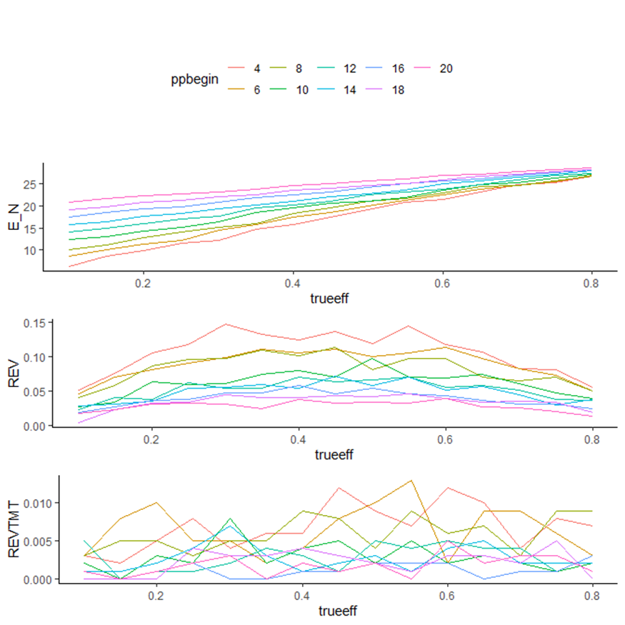
\(\mathbf{\tau}\mathbf{=}\mathbf{0.52}\), sample size equivalent=20
- Generate simulation dataset
# set seed
set.seed(125)

#   Proportion of responders to be observed at final that will lead to a non-stop decision
Target <- 0.52

# iteration
iter <- 1000

# PP stop/start
PP_stop <- 30

# Equivalent sample size
ne <- 20

# Simulation
TR <- length(TrueEffRange)

# Initiate parameters/data containers to be used in simulations
SimDataFigB <-
  data.frame(matrix(NA, length(PPrange) * length(TrueEffRange) * iter, 5)) # create matrix container

colnames(SimDataFigB) <- c("ppbegin","trueeff","stopN","reverseflag","meettargt")

stop_N <- vector(mode = "numeric", length = iter)
reverse <- vector(mode = "numeric", length = iter)
revtmt <- vector(mode = "numeric", length = iter)

row <- 1

if (file.exists("SimDataFigB.RData")){
  load("SimDataFigB.RData")
} else {
  for (pstat in PPrange){
  for (a in 1:length(TrueEffRange)){
    for (b in 1:iter){
        tr_out <- PPtrials(N, Ni, ne, TrueEffRange[a], Target, pstat, PP_stop, MON_stop)

        # the number of patients before NO Continue decision is made during iter times of sim
        stop_N[b] <- tr_out[[1]]
        # pp and corresponding #pt during ppstart to ppstop
        tr_hist <- tr_out[[2]]
        # meeting target?
        tmtfl <- tr_out[[3]]

        # flag the combination of pp/pp_N after the timepoint where pp monitoring is stopped
        after_stop <- tr_hist[tr_hist$PP1_N > stop_N[b],]
        # flag the reverse; but why stop_N[b] < PP_stop - 2 ????
        reverse[b] <- ifelse(length(after_stop[(after_stop$PP1 >= MON_stop),][,2]) == 0, 0, 1)
        # Number of times PP > MON_stop at end of monitoring | at least one reverse
        revtmt[b] <- ifelse(reverse[b]==1 & tmtfl==1, 1, 0)

        # package data.frame
        SimDataFigB[row,1] <- pstat
        SimDataFigB[row,2] <- TrueEffRange[a]
        SimDataFigB[row,3] <- stop_N[b]
        SimDataFigB[row,4] <- reverse[b]
        SimDataFigB[row,5] <- revtmt[b]

        row <- row+1
        }
  }
}

SimDataFigB[,1] <- as.factor(SimDataFigB[,1])
  save(SimDataFigB,file = "SimDataFigB.RData")
}- Analysis and plot
# Avg sample size
AnalyAvgSS_B <- SimDataFigB %>%
  group_by(ppbegin,trueeff) %>%
  summarise(E_N=mean(stopN)) %>%
  arrange(ppbegin,trueeff)

p_B1 <- ggplot(AnalyAvgSS_B, aes(x=trueeff, y=E_N, group=ppbegin)) +
  geom_line(aes(color=ppbegin))+
  theme_classic() +
  theme(legend.position = "none")

# Reversal
AnalyRev_B <- SimDataFigB %>%
  group_by(ppbegin,trueeff) %>%
  summarise(REV=mean(reverseflag)) %>%
  arrange(ppbegin,trueeff)

p_B2 <- ggplot(AnalyRev_B, aes(x=trueeff, y=REV, group=ppbegin)) +
  geom_line(aes(color=ppbegin))+
  theme_classic() +
  theme(legend.position = "none")

# Reversal + trial meets target
AnalyTmt_B <- SimDataFigB %>%
  group_by(ppbegin,trueeff) %>%
  summarise(REVTMT=mean(meettargt)) %>%
  arrange(ppbegin,trueeff)

p_B3 <- ggplot(AnalyTmt_B, aes(x=trueeff, y=REVTMT, group=ppbegin)) +
  geom_line(aes(color=ppbegin))+
  theme_classic() +
  theme(legend.position = "none")

# overall
grid.arrange(legend, p_B1, p_B2, p_B3, nrow = 4)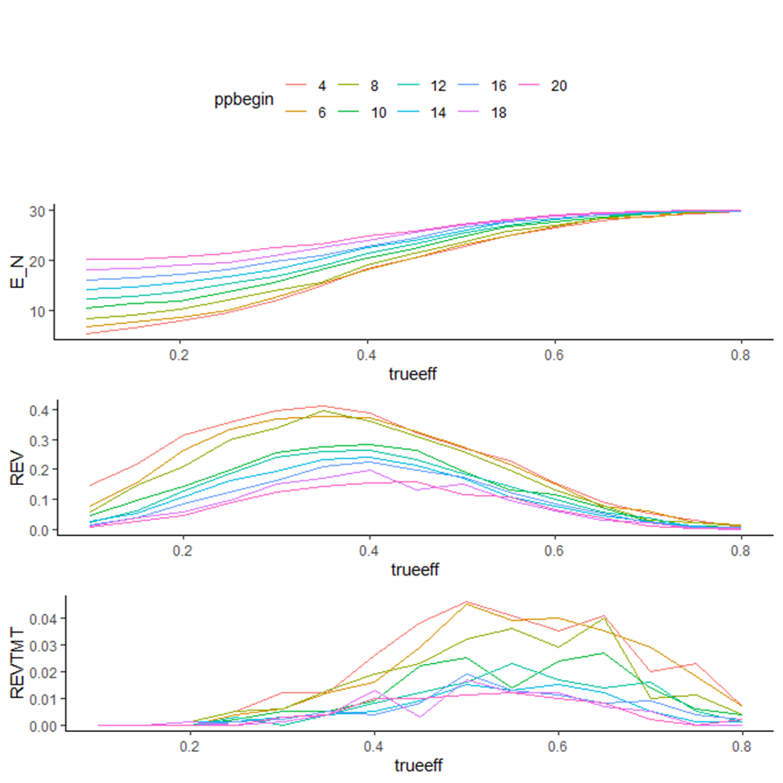
\(\mathbf{\tau}\mathbf{=}\mathbf{0.40}\), sample size equivalent=1
- Generate simulation dataset
# set seed
set.seed(125)

#   Proportion of responders to be observed at final that will lead to a non-stop decision
Target <- 0.40

# iteration
iter <- 1000

# PP stop/start
PP_stop <- 30

# Equivalent sample size
ne <- 1

# Simulation
TR <- length(TrueEffRange)

# Initiate parameters/data containers to be used in simulations
SimDataFigC <-
  data.frame(matrix(NA, length(PPrange) * length(TrueEffRange) * iter, 5)) # create matrix container

colnames(SimDataFigC) <- c("ppbegin","trueeff","stopN","reverseflag","meettargt")

stop_N <- vector(mode = "numeric", length = iter)
reverse <- vector(mode = "numeric", length = iter)
revtmt <- vector(mode = "numeric", length = iter)

row <- 1

if (file.exists("SimDataFigC.RData")){
  load("SimDataFigC.RData")
} else {
  for (pstat in PPrange){
  for (a in 1:length(TrueEffRange)){
    for (b in 1:iter){
        tr_out <- PPtrials(N, Ni, ne, TrueEffRange[a], Target, pstat, PP_stop, MON_stop)

        # the number of patients before NO Continue decision is made during iter times of sim
        stop_N[b] <- tr_out[[1]]
        # pp and corresponding #pt during ppstart to ppstop
        tr_hist <- tr_out[[2]]
        # meeting target?
        tmtfl <- tr_out[[3]]

        # flag the combination of pp/pp_N after the timepoint where pp monitoring is stopped
        after_stop <- tr_hist[tr_hist$PP1_N > stop_N[b],]
        # flag the reverse; but why stop_N[b] < PP_stop - 2 ????
        reverse[b] <- ifelse(length(after_stop[(after_stop$PP1 >= MON_stop),][,2]) == 0, 0, 1)
        # Number of times PP > MON_stop at end of monitoring | at least one reverse
        revtmt[b] <- ifelse(reverse[b]==1 & tmtfl==1, 1, 0)

        # package data.frame
        SimDataFigC[row,1] <- pstat
        SimDataFigC[row,2] <- TrueEffRange[a]
        SimDataFigC[row,3] <- stop_N[b]
        SimDataFigC[row,4] <- reverse[b]
        SimDataFigC[row,5] <- revtmt[b]

        row <- row+1
        }
  }
}

SimDataFigC[,1] <- as.factor(SimDataFigC[,1])
  save(SimDataFigC,file = "SimDataFigC.RData")
}- Analysis and plot
    # Avg sample size
    AnalyAvgSS_C <- SimDataFigC %>%
      group_by(ppbegin,trueeff) %>%
      summarise(E_N=mean(stopN)) %>%
      arrange(ppbegin,trueeff)

    p_C1 <- ggplot(AnalyAvgSS_C, aes(x=trueeff, y=E_N, group=ppbegin)) +
      geom_line(aes(color=ppbegin))+
      theme_classic() +
      theme(legend.position = "none")

    # Reversal
    AnalyRev_C <- SimDataFigC %>%
      group_by(ppbegin,trueeff) %>%
      summarise(REV=mean(reverseflag)) %>%
      arrange(ppbegin,trueeff)

    p_C2 <- ggplot(AnalyRev_C, aes(x=trueeff, y=REV, group=ppbegin)) +
      geom_line(aes(color=ppbegin))+
      theme_classic() +
      theme(legend.position = "none")

    # Reversal + trial meets target
    AnalyTmt_C <- SimDataFigC %>%
      group_by(ppbegin,trueeff) %>%
      summarise(REVTMT=mean(meettargt)) %>%
      arrange(ppbegin,trueeff)

    p_C3 <- ggplot(AnalyTmt_C, aes(x=trueeff, y=REVTMT, group=ppbegin)) +
      geom_line(aes(color=ppbegin))+
      theme_classic() +
      theme(legend.position = "none")

    # overall
    grid.arrange(legend,p_C1, p_C2, p_C3, nrow = 4)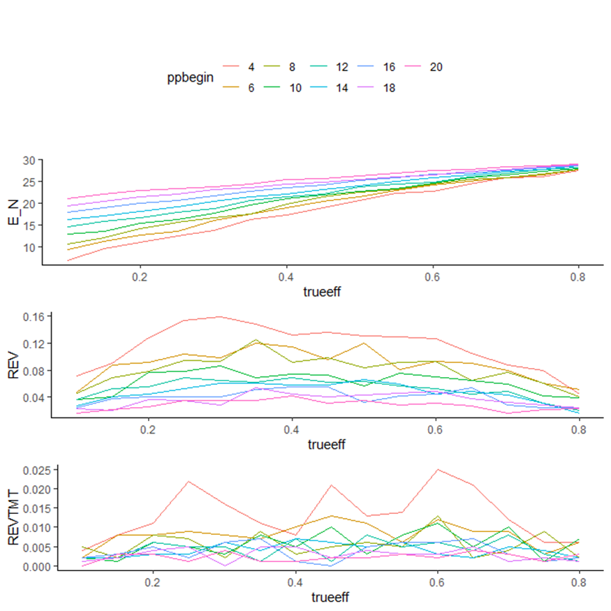
\(\mathbf{\tau}\mathbf{=}\mathbf{0.40}\), sample size equivalent=20
- Generate simulation dataset
# set seed
set.seed(125)

#   Proportion of responders to be observed at final that will lead to a non-stop decision
Target <- 0.40

# iteration
iter <- 1000

# PP stop/start
PP_stop <- 30

# Equivalent sample size
ne <- 20

# Simulation
TR <- length(TrueEffRange)

# Initiate parameters/data containers to be used in simulations
SimDataFigD <-
  data.frame(matrix(NA, length(PPrange) * length(TrueEffRange) * iter, 5)) # create matrix container

colnames(SimDataFigD) <- c("ppbegin","trueeff","stopN","reverseflag","meettargt")

stop_N <- vector(mode = "numeric", length = iter)
reverse <- vector(mode = "numeric", length = iter)
revtmt <- vector(mode = "numeric", length = iter)

row <- 1

if (file.exists("SimDataFigD.RData")){
  load("SimDataFigD.RData")
} else {
  for (pstat in PPrange){
  for (a in 1:length(TrueEffRange)){
    for (b in 1:iter){
        tr_out <- PPtrials(N, Ni, ne, TrueEffRange[a], Target, pstat, PP_stop, MON_stop)

        # the number of patients before NO Continue decision is made during iter times of sim
        stop_N[b] <- tr_out[[1]]
        # pp and corresponding #pt during ppstart to ppstop
        tr_hist <- tr_out[[2]]
        # meeting target?
        tmtfl <- tr_out[[3]]

        # flag the combination of pp/pp_N after the timepoint where pp monitoring is stopped
        after_stop <- tr_hist[tr_hist$PP1_N > stop_N[b],]
        # flag the reverse; but why stop_N[b] < PP_stop - 2 ????
        reverse[b] <- ifelse(length(after_stop[(after_stop$PP1 >= MON_stop),][,2]) == 0, 0, 1)
        # Number of times PP > MON_stop at end of monitoring | at least one reverse
        revtmt[b] <- ifelse(reverse[b]==1 & tmtfl==1, 1, 0)

        # package data.frame
        SimDataFigD[row,1] <- pstat
        SimDataFigD[row,2] <- TrueEffRange[a]
        SimDataFigD[row,3] <- stop_N[b]
        SimDataFigD[row,4] <- reverse[b]
        SimDataFigD[row,5] <- revtmt[b]

        row <- row+1
        }
  }
}

SimDataFigD[,1] <- as.factor(SimDataFigD[,1])
  save(SimDataFigD,file = "SimDataFigD.RData")
}- Analysis and plot
# Avg sample size
AnalyAvgSS_D <- SimDataFigD %>%
  group_by(ppbegin,trueeff) %>%
  summarise(E_N=mean(stopN)) %>%
  arrange(ppbegin,trueeff)

p_D1 <- ggplot(AnalyAvgSS_D, aes(x=trueeff, y=E_N, group=ppbegin)) +
  geom_line(aes(color=ppbegin))+
  theme_classic()+
  theme(legend.position = "none")

# Reversal
AnalyRev_D <- SimDataFigD %>%
  group_by(ppbegin,trueeff) %>%
  summarise(REV=mean(reverseflag)) %>%
  arrange(ppbegin,trueeff)

p_D2 <- ggplot(AnalyRev_D, aes(x=trueeff, y=REV, group=ppbegin)) +
  geom_line(aes(color=ppbegin))+
  theme_classic() +
  theme(legend.position="none")

# Reversal + trial meets target
AnalyTmt_D <- SimDataFigD %>%
  group_by(ppbegin,trueeff) %>%
  summarise(REVTMT=mean(meettargt)) %>%
  arrange(ppbegin,trueeff)

p_D3 <- ggplot(AnalyTmt_D, aes(x=trueeff, y=REVTMT, group=ppbegin)) +
  geom_line(aes(color=ppbegin))+
  theme_classic() +
  theme(legend.position="none")

# overall
grid.arrange(legend, p_D1, p_D2, p_D3, nrow = 4)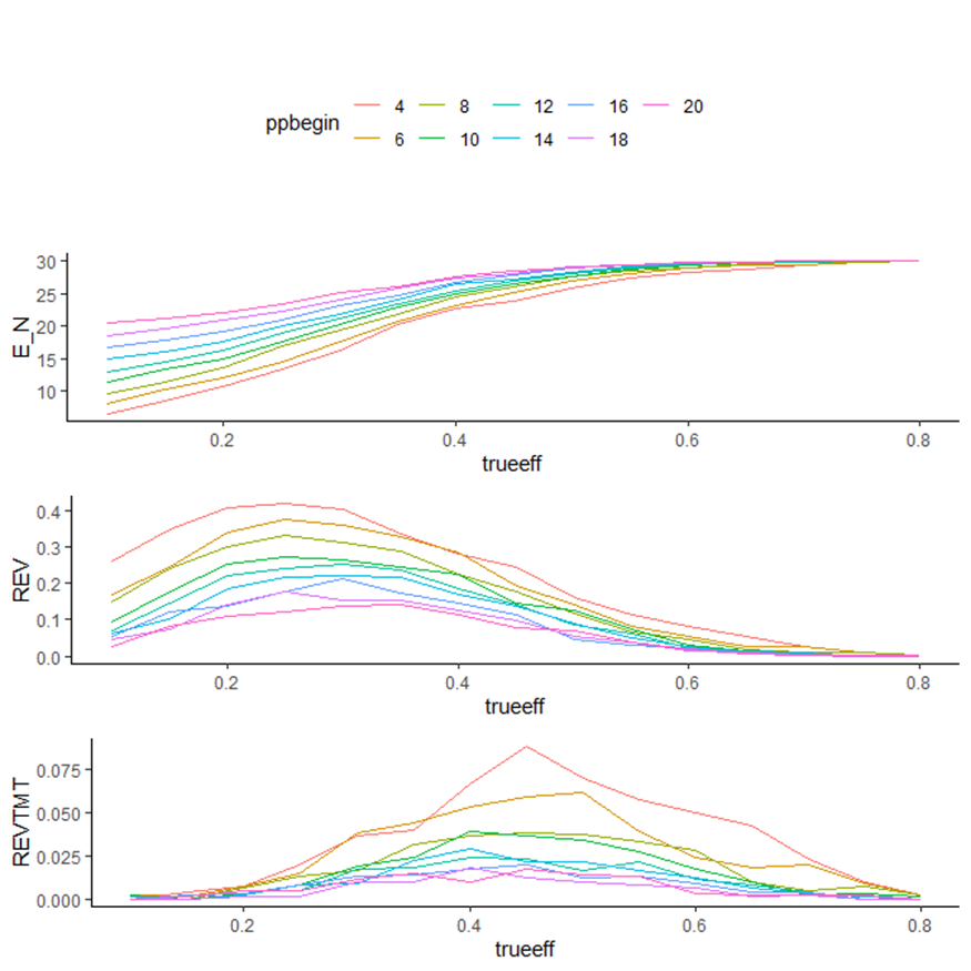
Guidance and Practical Implications
Setting \(\mathbf{\tau}\)
There are two considerations regarding the choice of \(\tau\).
- The first is that while \(\tau\) can relate to the choice of particular decision criteria at the end of the trial, in some cases this can lead to unacceptable operating characteristics.
- In particular, setting \(\tau\) too high can result in an unacceptably high probability of premature stopping.
Setting \(\tau\) higher than the target of interest is not recommended and will lead to discarding what would otherwise be good candidates for further development.
In the example above \(\tau\) is set according to the observed proportion of responders required out of the full planned sample that will lead to a non-stop decision at that point.
When comparing Table 3 (\(\tau = 0.52\)) and Table 4 (\(\tau = 0.40\)) the losses Pre IA and IA or before are the same when \(\tau = 0.52\). This suggests that there may be a point in any similar design where for \(\tau\) of at least some value, that all of the futility related decision making could be made based on the predictive probability monitoring.
An administrative look could then be incorporated if there is a desire to include a program decision that allows acceleration of planning or other activity within the program but outside the trial.
However, setting \(\tau\) too high can lead to an increase of inconsistent early stopping.
So, while \(\tau = 0.52\) was chosen as the non-stop criterion at the final analysis, it is not automatically set in this way. As with the values of any of the parameters, the operating characteristics of the corresponding design should be carefully understood before trial conduct.
TV/LRV and the lack of “PAUSE” results
With the decision framework that is used in these examples there are only two decision categories (GO/STOP). Results falling into one of these two categories suggest a clear basis for either continuing development or stopping development respectively.
With designs that include fewer patients or where the TV and LRV are set closer together, there can be a third decision category between the GO and STOP categories (PAUSE).
Results falling into this category are not by themselves enough to decide. This third category has typically meant that additional information from the trial should be considered in order to support a clear STOP or GO decision.
Reference
Lalonde RL, Kowalski KG, Hutmacher MM, et al. Model–based Drug Development. Clinical Pharmacology & Therapeutics. 2007;82(1):21–32.
Frewer P, Mitchell P, Watkins C, et al. Decision Making in Early Clinical Drug Development. Pharmaceutical Statistics. 2016;15(3):255–263.
The effect of the timing of beginning predictive probability monitoring
Selecting the beginning of the predictive probability monitoring phase of the design does have an impact on some of its operating characteristics (Figure 4).
The effect on average sample size is obvious and more pronounced in trials which terminate early since a certain number of patients are observed before the beginning of the predictive probability monitoring phase. Beyond this, average sample sizes rise to the maximum planned sample size with increasing True Effect mean.
The chance of observing a reversal increases with fewer patients observed before the predictive probability monitoring phase begins.
Further in this design there another decision point at the end of the trial that would have to be met before a compound would proceed further controlling the probability of an ineffective compound proceeding in development with borderline interim results. Though it is not something that was explored explicitly here, simulations are the best way to examine the effect of the start of the predictive probability phase of the trial on the overall risk of stopping the trial at various phases (looking specifically at the difference between the chance to stop without interim analysis and the corresponding chance to stop before IA, at IA or before or at any time in the trial).
Practical implications
In order for this method to be successfully implemented, strict adherence to the design as planned is necessary.
Changes to the timing of the start of any of the phases within the design are possible but would require simulations to fully understand the changes in the risks from the base case. This is necessary in order to avoid missing reversals in the response proportion. A reversal is suggestive of a STOP decision and should be taken seriously since the true mean proportion of patients responding is likely much lower than may otherwise be suggested when ignoring the reversal. This can lead to higher costs and more patients exposed to an otherwise ineffective compound than necessary.
It is also important to note that good ongoing data management is vital to the success of this design in particular when considering the possibility of stopping during the phase of the design concerned with the assessment of predictive probability. In particular, timely data entry and cleaning will quickly inform the possibility of a stop decision early in predictive probability monitoring. Changes in response due to data cleaning can increase the risk of incorrect decisions early and as an extension have unpredictable effects on average sample size.
As in all study designs, several assumptions are made for the purposes of planning the trial. In cases where more patients are recruited than originally planned, then as part of the procedures described in Frewer (2016) the criteria should be re-estimated with the current assumptions.
- Frewer P, Mitchell P, Watkins C, et al. Decision Making in Early Clinical Drug Development. Pharmaceutical Statistics. 2016;15(3):255–263.
Multiplicity
It is the case that in these examples there are 20 tests (predictive probability after patients 12–29 an interim at patient 30 and the final at patient 50) being conducted.
Were this trial to be designed using frequentist methods, there would be quite a number of adjustments made along with stopping boundaries specified for each of the 20 assessments.
Using Bayesian methodology and simulations, there is a much simpler way to address the problem. The operating characteristics are fully characterized over a number of True Effect distributions in terms of both sample size equivalents and range of True Effect mean. Since predictive probability is calculated using an algorithm, there is no need to calculate the individual stopping boundaries and include those in a protocol ahead of time. The algorithm is simply run following each patient until either a decision to stop the trial is made or until the planned number of patients in the predictive probability monitoring phase is reached.
Even though simulations are used along with an algorithm to estimate the chance of inappropriate early stopping, it is important to note that with more interim analyses (or longer periods of predictive probability monitoring), the risk of inappropriate stopping will increase.
Multiple simulations may be needed to select design parameters that lead to an acceptable level of risk.