In single-variable calculus, the second derivative \(f''(x)\) tells us about the curvature of a function:
\(f''(x) > 0\): function curves upward (convex locally)
\(f''(x) < 0\): function curves downward (concave locally)
\(f''(x) = 0\): possible inflection point
The Hessian matrix is the multivariable generalization of the second derivative. It captures curvature information in all directions simultaneously.
Why Does This Matter?
Single Variable
Multivariable
\(f''(x) > 0\) at critical point → local minimum
\(\mathbf{H}_f(\mathbf{x}) \succ 0\) at critical point → local minimum
\(f''(x) > 0\) everywhere → convex function
\(\mathbf{H}_f(\mathbf{x}) \succeq 0\) everywhere → convex function
\(f''(x) < 0\) at critical point → local maximum
\(\mathbf{H}_f(\mathbf{x}) \prec 0\) at critical point → local maximum
2. Definition of the Hessian Matrix
Definition (Hessian Matrix)
Let \(f: \mathbb{R}^n \to \mathbb{R}\) be a twice continuously differentiable function. The Hessian matrix of \(f\) at point \(\mathbf{x} \in \mathbb{R}^n\) is the \(n \times n\) matrix of second-order partial derivatives:
Note: The Hessian is constant (independent of \(\mathbf{x}\)) for quadratic functions. This is why quadratic functions are the “simplest” case for optimization analysis.
Higher-order terms (negligible for small \(\mathbf{d}\))
Directional Curvature
The term \(\mathbf{d}^\top \mathbf{H}_f(\mathbf{x}) \mathbf{d}\) captures how the function curves in direction \(\mathbf{d}\).
Definition (Directional Second Derivative):
For a unit vector \(\mathbf{u}\) (\(\|\mathbf{u}\| = 1\)), the second directional derivative of \(f\) at \(\mathbf{x}\) in direction \(\mathbf{u}\) is:
Since computing and inverting the Hessian is expensive, quasi-Newton methods build an approximation \(\mathbf{B}_k \approx \mathbf{H}_f(\mathbf{x}_k)\) iteratively.
Key property: If \(f\) is convex (so the true Hessian is PSD), and certain conditions hold, the BFGS approximation remains PD, ensuring descent directions.
7.4 When the Hessian is Not PD
If \(\mathbf{H}_f(\mathbf{x}_k)\) is not positive definite (e.g., near a saddle point), Newton’s direction may not be a descent direction.
Solutions:
Modified Newton: Replace \(\mathbf{H}\) with \(\mathbf{H} + \lambda \mathbf{I}\) where \(\lambda > 0\) makes it PD
Trust Region Methods: Restrict step size to region where quadratic model is valid
Line Search: Ensure sufficient decrease along the Newton direction
8. Applications in Statistics and Machine Learning
8.1 Maximum Likelihood Estimation (MLE)
For log-likelihood \(\ell(\boldsymbol{\theta})\), we want to find:
where \(\mathbf{W} = \text{diag}(p_1(1-p_1), \ldots, p_n(1-p_n))\)
Key insight: Since \(0 < p_i < 1\), we have \(p_i(1-p_i) > 0\), so \(\mathbf{W} \succ 0\). Thus \(\mathbf{H}_\ell \prec 0\), meaning the log-likelihood is concave and has a unique maximum!
8.3 Neural Networks and Non-Convexity
Neural network loss functions are typically non-convex:
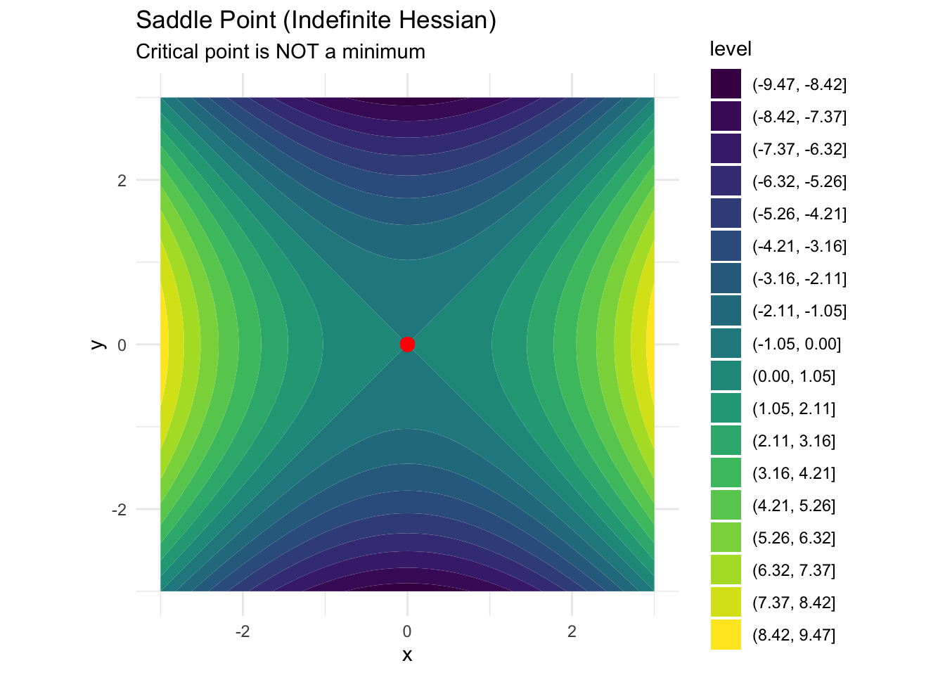
The Hessian can be indefinite (saddle points are common)
Multiple local minima exist
Gradient descent can get stuck
Role of the Hessian in deep learning:
Understanding loss landscape: Eigenvalues of Hessian reveal curvature structure
This requires \(-\mathbf{H}_\ell\) to be positive definite (i.e., \(\ell\) is concave at the MLE).
Standard errors:\(\text{SE}(\hat{\theta}_j) = \sqrt{[\mathbf{I}(\hat{\boldsymbol{\theta}})^{-1}]_{jj}}\)
9. Computational Considerations
9.1 Checking Positive Definiteness
Methods to check if \(\mathbf{H}\) is PD:
Method
Complexity
Notes
Compute all eigenvalues
\(O(n^3)\)
Check if all \(\lambda_i > 0\)
Cholesky decomposition
\(O(n^3/3)\)
Succeeds iff PD
Leading principal minors
\(O(n^4)\)
Check if all positive
Sylvester’s criterion
\(O(n^4)\)
Compute \(n\) determinants
In practice: Try Cholesky decomposition. If it fails, the matrix is not PD.
9.2 Numerical Issues
Problem: Computed Hessian may not be exactly symmetric or PD due to: - Floating-point errors - Finite difference approximations - Numerical instability
Regularize:\(\mathbf{H} \leftarrow \mathbf{H} + \epsilon \mathbf{I}\) for small \(\epsilon > 0\)
Project to PSD cone: Use eigendecomposition, clip negative eigenvalues to zero (or small positive value)
9.3 Hessian-Free Methods
For large-scale problems, storing the \(n \times n\) H
Reference
Content generated by Claude (Claude Opus 4.5), an AI assistant developed by Anthropic. Conversation date: [Your Date]. Retrieved from: https://claude.ai/
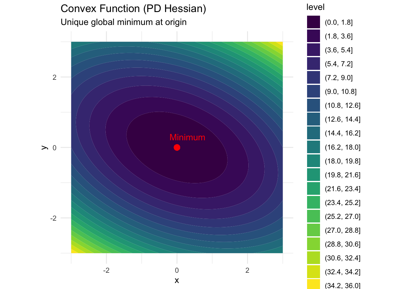
# -----------------------------------------------------------------------------# 3. VISUALIZE CONVEX FUNCTION# -----------------------------------------------------------------------------# Create contour plotgrid <-expand.grid(x =seq(-3, 3, 0.1), y =seq(-3, 3, 0.1))grid$z <-apply(grid, 1, f)ggplot(grid, aes(x, y, z = z)) +geom_contour_filled(bins =20) +geom_point(aes(x =0, y =0), color ="red", size =3) +annotate("text", x =0.3, y =0.3, label ="Minimum", color ="red") +labs(title ="Convex Function (PD Hessian)", subtitle ="Unique global minimum at origin") +theme_minimal() +coord_fixed()
# -----------------------------------------------------------------------------# 4. NEWTON'S METHOD# -----------------------------------------------------------------------------newton_method <-function(f, grad, hess, x0, tol =1e-8, max_iter =100) { x <- x0 history <-list(x)for (i in1:max_iter) { g <-grad(x) H <-hess(x)# Newton step: x_new = x - H^{-1} * g d <-solve(H, -g) x <- x + d history[[i +1]] <- xif (sqrt(sum(g^2)) < tol) break }list(minimum = x, iterations = i, path =do.call(rbind, history))}result <-newton_method(f, grad_f, hess_f, x0 =c(2, 2))cat("\nNewton's Method Result:\n")
# Visualize saddlegrid$z_saddle <-apply(grid[, 1:2], 1, f_saddle)ggplot(grid, aes(x, y, z = z_saddle)) +geom_contour_filled(bins =20) +geom_point(aes(x =0, y =0), color ="red", size =3) +labs(title ="Saddle Point (Indefinite Hessian)",subtitle ="Critical point is NOT a minimum") +theme_minimal() +coord_fixed()
# -----------------------------------------------------------------------------# 6. LOGISTIC REGRESSION EXAMPLE# -----------------------------------------------------------------------------# Simulate dataset.seed(42)n <-200X <-cbind(1, rnorm(n), rnorm(n))beta_true <-c(-0.5, 1.5, -1)p_true <-1/ (1+exp(-X %*% beta_true))y <-rbinom(n, 1, p_true)# Negative log-likelihood (to minimize)nll <-function(beta) { eta <- X %*% beta-sum(y * eta -log(1+exp(eta)))}# Gradientgrad_nll <-function(beta) { p <-1/ (1+exp(-X %*% beta))-t(X) %*% (y - p)}# Hessianhess_nll <-function(beta) { p <-1/ (1+exp(-X %*% beta)) W <-diag(as.vector(p * (1- p)))t(X) %*% W %*% X # Always PSD!}# Fit using Newton's methodbeta_hat <-newton_method(nll, grad_nll, hess_nll, x0 =c(0, 0, 0))$minimum
Warning in (function (..., deparse.level = 1) : number of columns of result is
not a multiple of vector length (arg 1)
cat("\nLogistic Regression Coefficients:\n")
Logistic Regression Coefficients:
cat("True:", beta_true, "\n")
True: -0.5 1.5 -1
cat("Estimated:", round(beta_hat, 3), "\n")
Estimated: -0.449 1.636 -1.771
# Verify Hessian is PDcat("\nHessian at MLE:", check_definiteness(hess_nll(beta_hat)), "\n")
Hessian at MLE: Positive Definite (Convex)
# Standard errors from inverse Hessianse <-sqrt(diag(solve(hess_nll(beta_hat))))cat("Standard Errors:", round(se, 3), "\n")