A Brief Introduction to Causal Inference
Abstract
Statistics has been highly successful in “correlation” but has had limited achievements in “causation.” This post begins with the Yule-Simpson Paradox to illustrate the difficulties of causal inference. It then introduces the Rubin Causal Model (RCM) and its application in randomized trials. It also discusses Principal Stratification and Instrumental Variables for handling complications. Finally, it introduces Causal Diagrams (DAGs), the do operator, and the Front-Door and Back-Door criteria for identifying causal effects.
This post is based on the document “An Introduction to Causal Inference” by Peng Ding from Peking University.
1. Correlation vs. Causation: The Yule-Simpson Paradox
The Yule-Simpson Paradox is a key example of why correlation does not imply causation.
The Paradox: A statistical association (e.g., positive correlation) observed in an aggregate population can be reversed when the population is divided into subgroups (strata). (also see FDA technical guidance: Adjusting for Covariates in Randomized Clinical Trials for Drugs and Biological Products [May 2023] )
Example (Table 1): A drug appears beneficial overall (50% recovery vs. 40% for placebo). However, when stratified by gender, the drug is harmful for both men (60% vs. 70%) and women (20% vs. 30%).
Why it Happens: This is due to a confounding variable (Gender) that is associated with both the treatment (Drug) and the outcome (Recovery). In epidemiology, this is known as “confounding bias”.
Implication: This paradox demonstrates the danger of drawing causal conclusions from observational data (e.g., smoking and lung cancer) without accounting for confounders.
2. Rubin Causal Model (RCM) and Randomized Trials
The Rubin Causal Model (RCM) provides a precise framework for defining causal effects.
Potential Outcomes: For each individual \(i\), we define two potential outcomes:
\(Y_i(1)\): The outcome if individual \(i\) receives the treatment.
\(Y_i(0)\): The outcome if individual \(i\) receives the control.
Individual Causal Effect (ICE): The causal effect for individual \(i\) is \(Y_i(1) - Y_i(0)\).
The Fundamental Problem for Individual Causal Effect: The ICE is unidentifiable because we can only observe one potential outcome for each individual (either \(Y_i(1)\) or \(Y_i(0)\), but never both. For a specific individual, his/her potential outcome is determined. Please note that for individual \(i\), the potential outcome is a definite value; the randomness here lies in individual \(i\), and \(i\) can be regarded as a sample point \(\omega\) in the sample space \(\Omega\) as defined in conventional probability theory.).
Average Causal Effect (ACE): While we cannot identify individual effects, we can aim to identify the Average Causal Effect (ACE) for the population:
\[ACE(Z \rightarrow Y) = E[Y_i (1) - Y_i(0)]\]
Role of Randomization: In a completely randomized trial, the treatment assignment \(Z\) (\(Z_i=1\) for receiving IP; \(Z_i=0\) for receiving control) is statistically independent of the potential outcomes (\(Z \perp (Y(1), Y(0))\)). This independence is the key.
Identification: Randomization allows us to estimate the ACE using observed data (See the arithmetic expression on the far right of the following equation), as the confounding bias is broken:
\[ACE(Z \rightarrow Y) = E[Y_i(1)] - E[Y_i(0)] = E[Y_i|Z_i=1] -[Y_i|Z_i=0]\]
3. Causal Inference in “Failed” Randomized Trials
In an ideal randomized trial, individuals in the treatment group (referred to as “IP”) and control group fully adhere to the assigned protocols.
However, in reality, participants in the trial may exhibit noncompliance, drop out early, or die before the outcome variables are observed (sometimes we may exclude such participants from Per-Protocol Analysis Set).
These situations give rise to three issues: noncompliance, non-random missing data, and death-censoring. Below is a separate introduction to noncompliance and death-censoring, while the problem of missing data exists in most statistical scenarios.
3.1 Noncompliance and Instrumental Variables
Problem: In a trial, subjects may not comply with their assigned treatment. We have:
\(Z\): The randomized assignment (Intent-to-Treat).
\(D\): The actual treatment received.
\(N\): The number of subjects in the population.
\(Y\): Potential outcome.
Noncompliance: \(Z_i \neq D_i\) (\(i\) for the index of a subject).
Invalid Analyses:
Intent-to-Treat (ITT): Analyzing \(E[Y|Z=1] - E[Y|Z=0]\). This estimates the causal effect of the randomized assignment, not the treatment itself.
As-Treated (AT): Analyzing \(E[Y|D=1] - E[Y|D=0]\). This is a confounded observational comparison, as \(D\) is not randomized; therefore, there exists confounding between \(D\) and \(Y\) (i.e., there may be common causes influencing both whether individual \(i\) receives the treatment and its outcome variable). Consequently, the difference in means between the two groups obtained does not represent the effect of the treatment.
Solution: Principal Stratification: We stratify the population based on their potential compliance behavior (Frangakis and Rubin(2002)), which is a pre-randomization attribute.
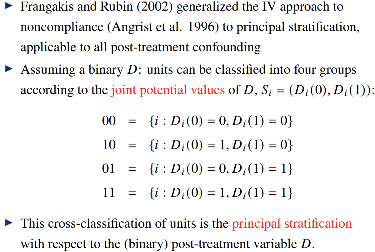
This creates four groups:
-   **Compliers:** Always follow assignment.

-   **Never-takers:** Always in control group.

-   **Always-takers:** Always in treatment group.

-   **Defiers:** Always do the opposite of assignment.
CACE / LATE: We can identify the Complier Average Causal Effect (CACE), also known as the Local Average Treatment Effect (LATE).
Identification: Under two key assumptions:
Monotonicity: There are no defiers.
Exclusion Restriction: The assignment \(Z\) only affects the outcome \(Y\) through the treatment \(D\).
Result: The CACE is identified by the Wald estimator, which is an Instrumental Variable (IV) estimate:
\(CACE = \frac{E[Y|Z=1]-E[Y|Z=0]}{E[D|Z=1]-E[D|Z=0]} = \frac{ACE(Z \to Y)}{ACE(Z \to D)}\)
4.2 Truncation by Death
Problem: If a treatment affects survival (\(S\)), the outcome of interest \(Y\) (e.g., quality of life) may be undefined for those who die (\(S=0\)). This is not a simple missing data problem.
Solution: Use Principal Stratification based on potential survival (\(S(1)\) and \(S(0)\)).
SACE: We can only define a meaningful causal effect for the “Always-Survivor” group (those who would survive under both treatment and control). This is the Survivor Average Causal Effect (SACE).
\[ SACE = E[Y(1) - Y(0) | S(1)=1, S(0)=1] \]
5. The Bayesian View of RCM
The RCM framework can be viewed from a Bayesian perspective, which treats causal inference as a missing data problem.
Framework: The unobserved potential outcome (\(Y(0)\) for a treated person, \(Y(1)\) for a control person) is the “missing data”.
Goal: The task is to “fill in” (predict) the posterior distribution of the missing potential outcomes given the observed data.
Ignorability: When the treatment assignment mechanism is ignorable (e.g., randomization), the inference for the causal effect simplifies and depends only on the model for the data, not the assignment mechanism.
Advantage: For problems that are not identifiable in the frequentist sense (e.g., noncompliance without the monotonicity assumption), the Bayesian approach can still provide an updated posterior distribution for the parameters, incorporating information from the data.