Basket Trial Design - A Simulated Study

mathematical statistics

sap

trial design

oncology

A basket trial is a type of clinical trial design used in oncology that tests the effectiveness of a single drug in treating multiple types of cancer that share a specific genetic mutation or biomarker, regardless of where the cancer originated in the body. It allows researchers to efficiently evaluate a targeted therapy across different cancer types.

Author

Yupng L.

Published

May 26, 2022

NOTE THAT THE FOLLOWING CODES ARE USED FOR DEMONSTRATING ONLY. THE EXECUTABLE CODES WILL NOT BE ATTACHED HERE. R IS THE TOOL FOR BAYESIAN HIERARCHICAL MODELING.

Background

Brief Summary

The purpose of this study is to evaluate the objective response rate (complete response [CR]+ partial response [PR]) of the selected dose regimen in participants with cancers that harbor specific genomic alterations.

Study Design

This is a multicenter, open-label study (participants will know the identity of study drugs administered) to evaluate the efficacy and safety of STUDY DRUG in participants with urothelial cancer.

The study comprises a 30-days Screening Phase, a Treatment Phase comprised of 28-day treatment cycles that will continue until specific event occurs, and a post-treatment Follow-up Phase that will extend from the End-of-Treatment Visit (EOT) until the participant has died, withdraws consent, is lost to follow-up, or the end of the study, whichever comes first.

Cohort

There are 15 tumor histologies in the basket trial. The Prevalence of tumor histology (3rd column in the following table) will be used in simulation when generating a patient with specific tumor histology.

Cancer Type	Target XX Frequency (%)	Anticipated Tumor Representation in Target XX+ Population plus “Other” Group (%)
a	21	18
b	4	18
c	9	13
d	3	13
e	2	10
f	11	5
g	7	4
h	5	4
i	2	3
j	8	2
k	1	2
l	3	1
m	1	1
n	2	1
o	1	-
other	-	5

Primary Outcome Measures

Percentage of Participants with Best Overall Response (ORR)

Seed

set.seed(123)

Core Parts in Simulation Settings

This code was developed as a personal exercise and has not been fully validated.

General statements

There will be 2 interim futility analyses and 1 final analysis when

datacut = c(60,130,200) # 200 is final analysis

During interim futility analyses, the futility criteria is: Less than a 40% chance that ORR>25%

\[ posterior \ P(ORR>0.25)<0.4 \]

During final analysis, two kinds of analyses will be performed:

BHM by using success criteria which is: Greater than an 80% chance that ORR >25%

\[ posterior \ P(ORR>0.25)>0.8 \]

Pooling efficacy analysis

Before pooling, a futility analysis with the futility criteria above at final efficacy analysis on all tumor histologies to decide the tumor agnostic pool and which histology should not succeed as a pool. An exact binomial test in the final pooled efficacy analysis with a null hypothesis $ORR=0.15$ and an alternative hypothesis $ORR>0.15$ at $\alpha=0.05$.

Enrollment pattern

# set the total sample size
ss <- 200

# set the cap for each cohort
cap <- 30

# set the accrual rate to 10/7 subjects/week
accrate = 10/7 <- 10/7

For each participant, we assume that a confirmed CR/PR is available after 28 days from their first tumor assessment.

trdur = 4*7

Cohort

The following process simulates the assignment to corresponding tumor histology.

Note that letters A to O will be used to represent the 15 tumor histology in simulation.

Input the proportion of each tumor histology for enrollment into the trial:

tumorprop = c(18,18,13,13,10,5,4,4,3,2,2,1,1,1,5)*0.01

Response

There are 6 different scenarios that are based on the assumed true ORR for each tumor histology. Six scenarios are shown, with different true ORRs for each histology.

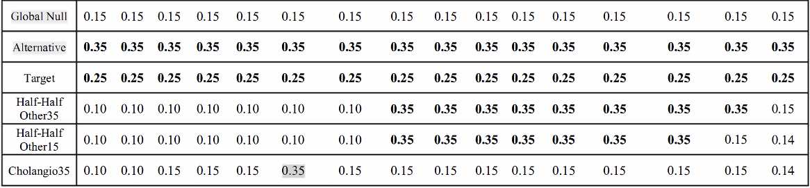
Different scenarios will be used to evaluate different operating characteristics which will be introduced later.

The Global Null scenario is to evaluate the false positive rate (FPR) for the final pooled efficacy analysis and the family-wise error rate (FWER) with BHM analysis.
The scenarios Alternative and Target are for power assessment.
The scenarios Half-Half Other35, Half-Half Other15, and Cholangio35, with their original tumor agnostic pooled ORR at the null, are designed to assess the impact of futility and to evaluate the FPR for final pooled efficacy analysis.

Operating characteristics

BHM analysis

Selection power

Selection power is the proportion of simulations that selected at least a given percentage of active tumor histologies (e.g. 80%) to be pooled for final efficacy analysis.

Proportion of success

Proportion of success is the proportion of simulations in which BHM claimed at least one tumor histology as a success. Similarly, the success criteria $(Pr(ORR > 25\%) > 80\% )$ is used for BHM to claim a success (efficacy) for a given tumor histology.

Family-wise Error Rate (FWER)

FWER represents the proportion of simulations in which BHM claimed false-positive efficacy in one or more of the nonactive tumor histologies. Note that the success criteria $(Pr(ORR > 25\%) > 80\%)$ is used for BHM to claim a success (efficacy) for a given tumor histology.

Pooled efficacy analysis

Power

Power is calculated as the proportion of simulations claiming a success (efficacy) on the Pooled data of final efficacy analysis. Note that a futility analysis should be perform to decide which histology will be succeed in pooled efficacy analysis.

False positive rate (FPR)

FPR is defined as the proportion of simulations claiming a false-positive success (efficacy) on the pooled data of final efficacy analysis. Note that a success is false-positive only when the weighted average of true ORRs is less than 15% (It should be <= 15% in practice) for the remaining histologies that didn’t meet the futility criteria in the final pool for efficacy analysis. The weights are the renormalized assumed prevalence in for each tumor histology that ended up in the final pool.

Mixing non-active

Mixing nonactive is defined as the proportion of claiming a success (efficacy) in the pooled data at the final efficacy analysis that is mixed with at least one nonactive histology.

General consideration in implementation

5000 simulation runs will be conducted to evaluate the operating characteristics of the proposed design.

Simulated data generation

For 1st interim analysis

Specify an multiplier $multiplier=3$. A total of 60 records should be used in 1st interim futility analysis, therefore we generate $60*multiplier=180$ records. e.g.

multiplier = 3

Generate histology, response, relative enrollment day, confirmed PR/CR day for each record (participant);
Create a counter to check if the sample size of a histology reaches the cap. If yes, the recruitment for this histology will be stopped.
Flag all qualifying 60 records for 1st interim analysis) and those records with relative enrollment day <= the maximum relative enrollment day (in those 60 participants) + 28 days for 2nd interim analysis.
Delete all other records unflagged.

For $x$ ($x>1$) interim analysis

Generally follow the ideas described in 1. But for those histology that does not pass the 1st interim futility analysis, recruitment will be also stopped in this kind of cohort.

Bayesian model

Note that, the way of implementing the generation of the following random numbers is different from that in RJAGS. The following contents in this part are provided for illustration purpose.

Denote $\pi_g=Pr(response \mid treatment, g)$, the BHM models the log-odds response (i.e. ORR)

defined as

$$ _g=logit(_g)=

\[ with weak prior \]

_g N(,^2) \ N(-2.19,2^2) $$

And $^2 $ Inverse Gamma with mean 2 and weight 0.75.

Some points need to be noticed:

In implementation, we need to make a transform on log-odds of response

\[ \pi_g=\frac{exp(\theta_g)}{1+exp(\theta_g)} \]

Inverse Gamma distribution with mean 2 and weight 0.75 could be visualized as

library(invgamma)

# generate the hyper-parameters for tau^2 by inverse gamma
Tau2_ab <- function(mean,weight){
  a <- weight/2
  b <- (mean^2)*weight/2
  return(c(a,b))
}

# call the function and validate by visualization
invgamma_input <- Tau2_ab(2,0.75)
x_dinvgamma <- seq(0, 10, by = 0.01)   

# Apply dinvgamma function
y_dinvgamma <- dinvgamma(x_dinvgamma,invgamma_input[1],invgamma_input[2]) 

# Plot tau^2
plot(x_dinvgamma,y_dinvgamma,type="l")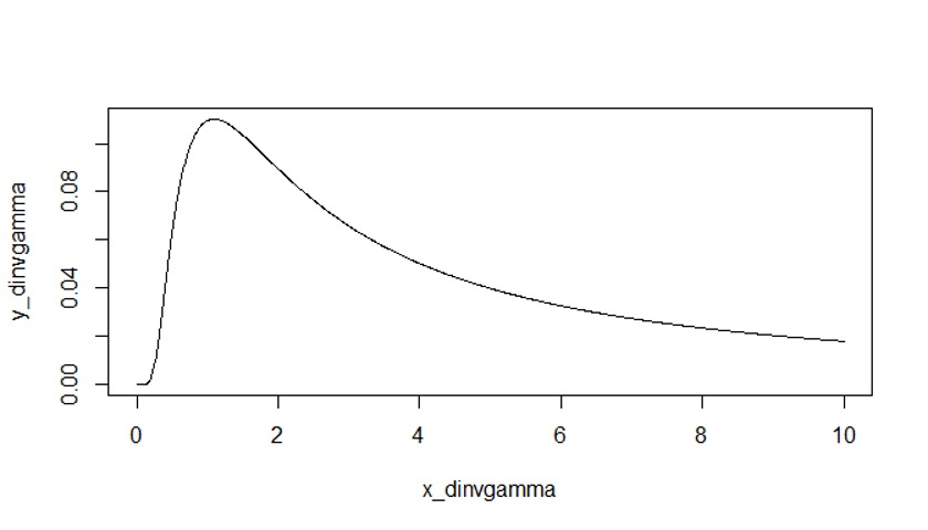

For the setting of hierarchical modeling in RJAGS, the 2nd parameter in dnorm(mean,precision) is precision instead of variance or standard deviation.
The overall bayesian calculation looks like the following codes. We need to set a number for burn-in chains in order to get a Markov Chain reaches its equilibrium distribution.

  # set burn in
  burn.in = 2000
  
  # DEFINE the BH model
  bayes_model <- "model{
    # Likelihood model for PiG
    for (i in 1:length(K)){
      K[i] ~ dbin(orr[i],n[i])
      orr[i] <- exp(thetag[i])/(1+exp(thetag[i]))
    }
    for (i in 1:length(K)){
      thetag[i] ~ dnorm(mu,tau2)
    }

    # Prior model for thetag,mu,tau2
    mu ~ dnorm(a, b)
    # sigma2 <- 1/tau2
    ## inverse gamma
    tau2 ~ dgamma(alpha,beta)
    }"
  
  bayes_jags_IA <- jags.model(
    textConnection(bayes_model),
    data = list(
      a = a,
      b = b,
      K = summary_adam$responders,
      alpha = invg_a,
      beta = invg_b,
      n = summary_adam$n
    ),
    inits = list(.RNG.name = "base::Wichmann-Hill", .RNG.seed = mcmc_seed),
    quiet = TRUE
  )
  # mcmc to generate the posterior
  update(bayes_jags_IA, burn.in)
  bayes_sim_IA <-
    coda.samples(model = bayes_jags_IA,
                 variable.names = c("orr"),
                 n.iter = mcmc_iter)
  # Store the chains in a matrix -- source of posterior of orr
  bayes_chains_IA <- bayes_sim_IA[[1]]

Pooled analysis model

An exact binomial test should be performed on the histologies that succeed in the futility analysis before pooling.

pooltotalresp is the number of total responders in the histologies being pooled;

poolsamplesize is the number of total sample size in the histologies being pooled.

p0 is 0.15 in this case.

binom.test(x=pooltotalresp,n=poolsamplesize,p=p0,alternative = "greater")

Results

The results are generated by invoking Analysis2.R. Results are represented as

A summary table of Operating Characteristics for FWER, FPR and etc..
Figures of Selection Power Plot for different Scenarios listed in this document.

Operating Characteristics

Selection Power

All15

All35

All25

Half Half 35

Half Half 15

Cholangio 35

Appendix

How to run the simulation

Put the 3 files in a same location

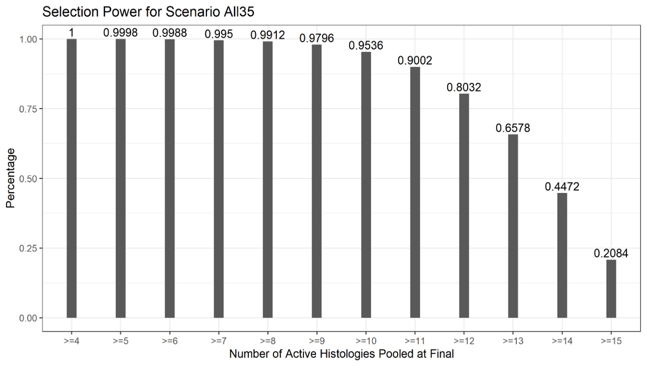
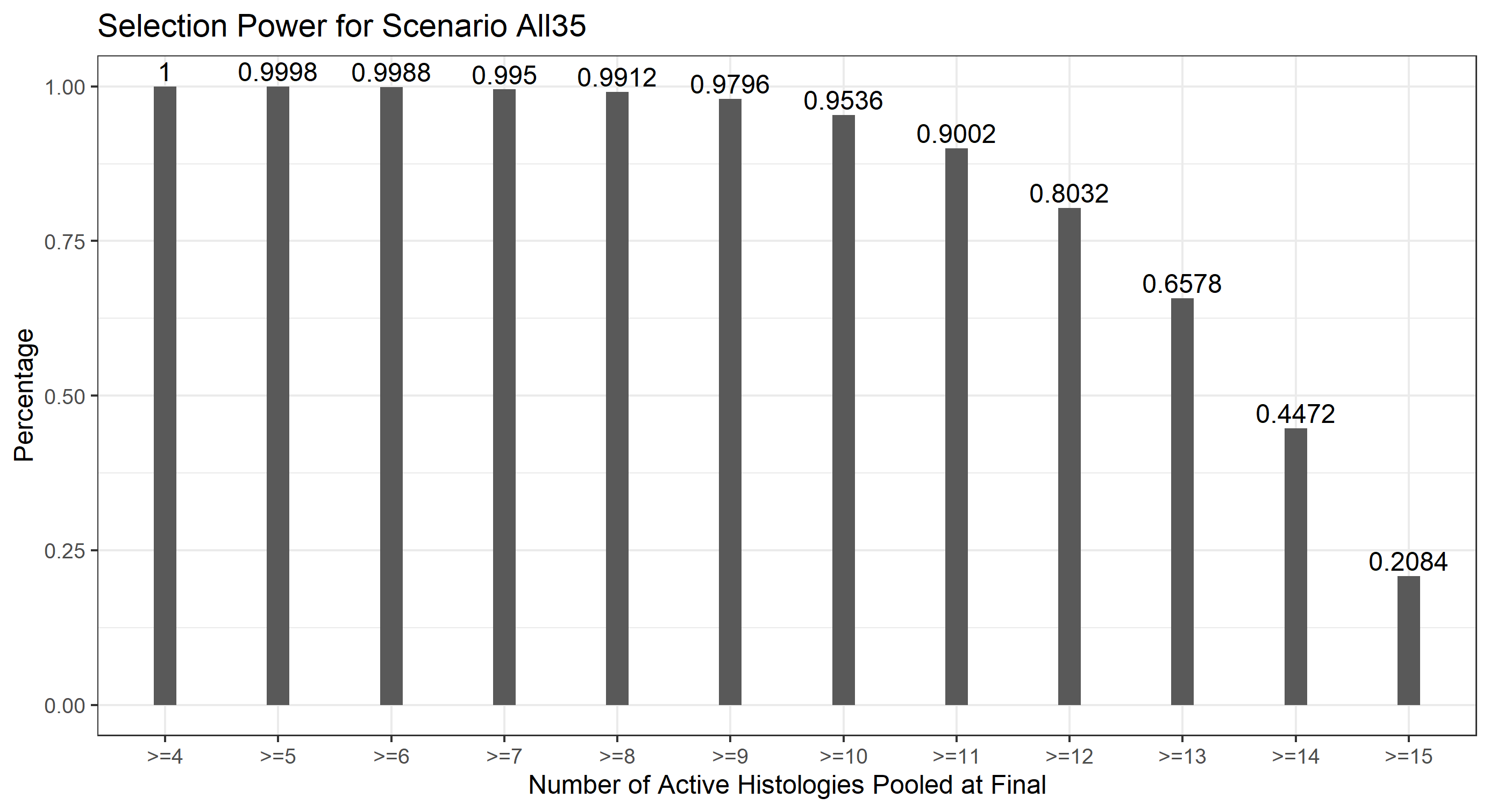
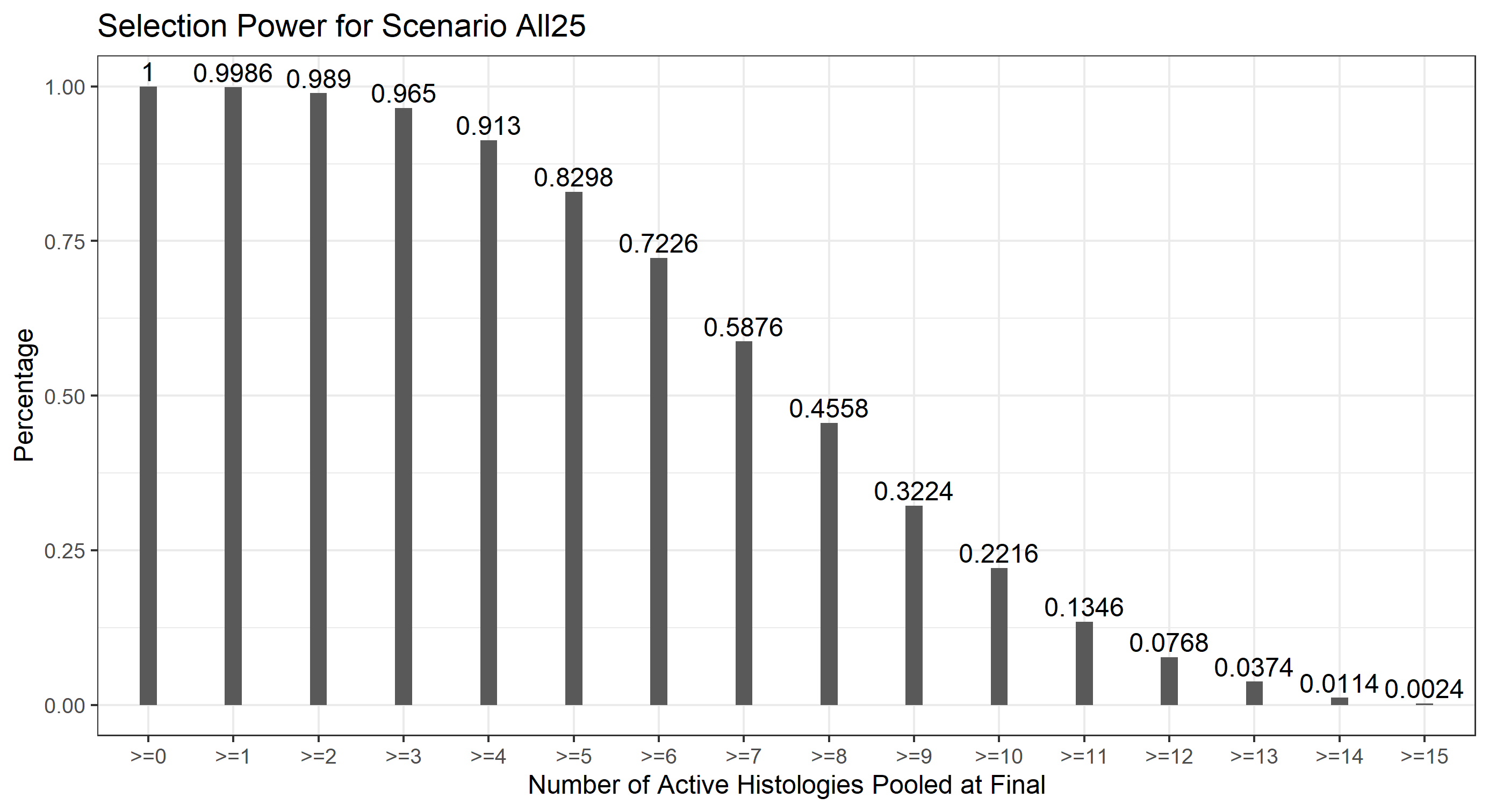
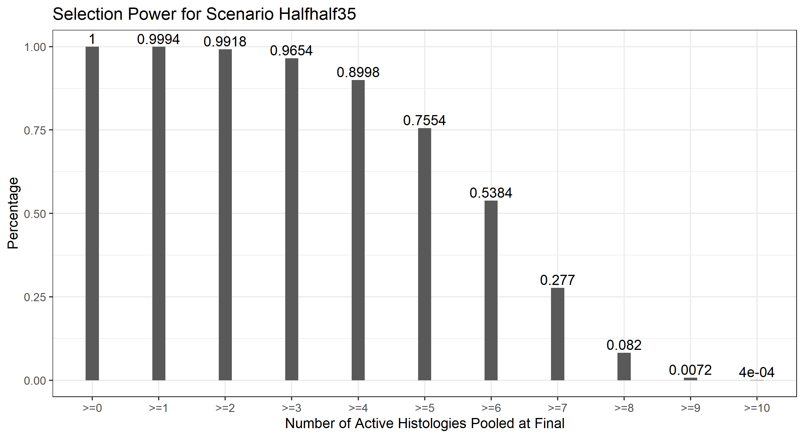
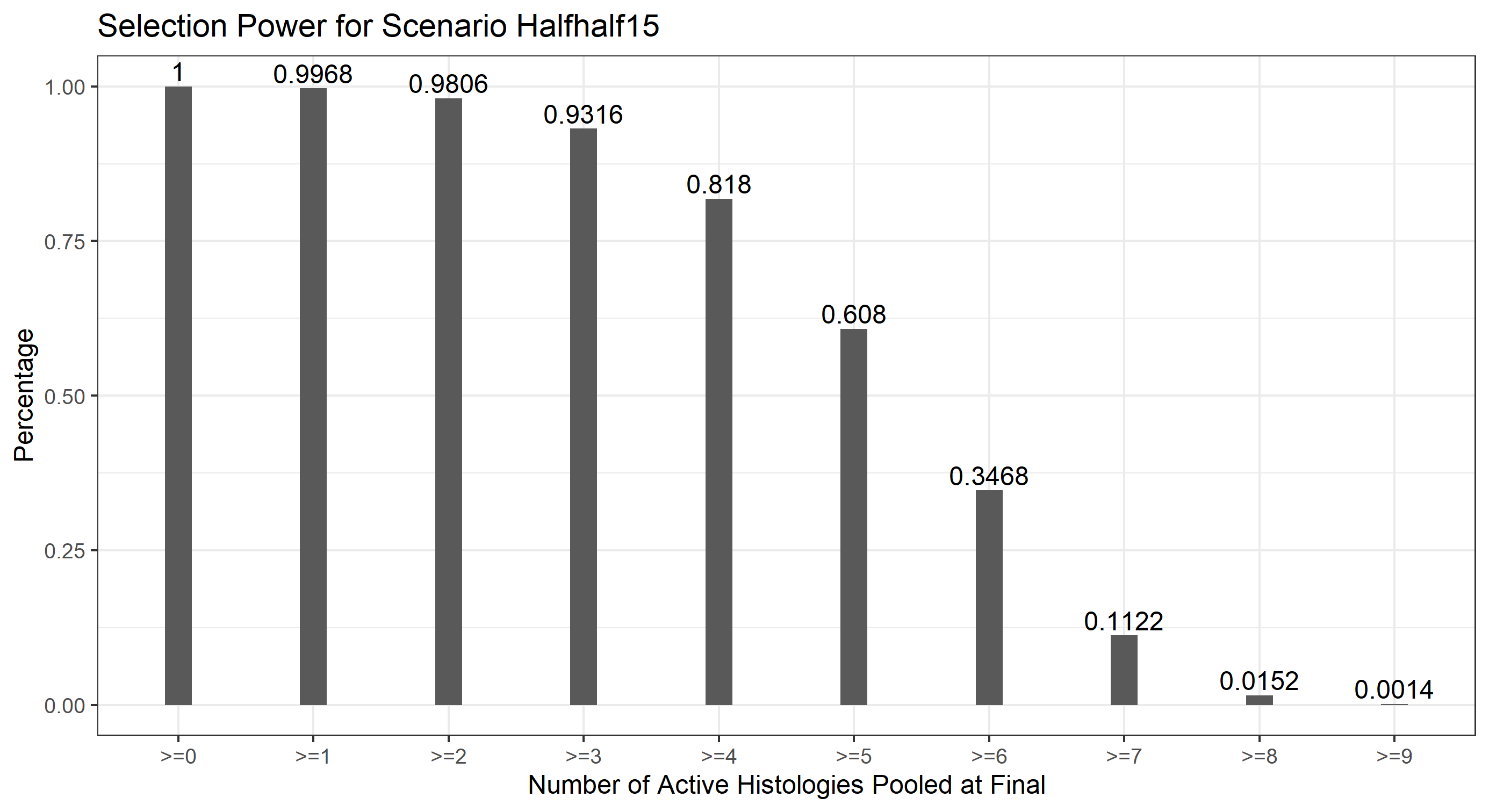
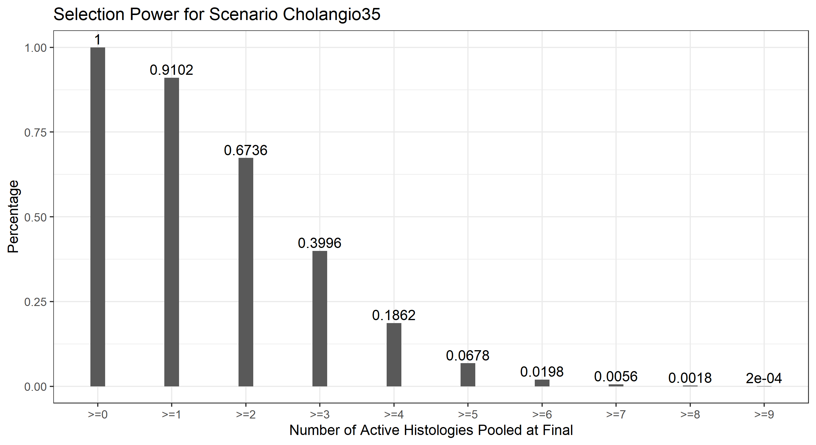
function2.R : contains utility functions and main functions to perform simulations
TrialSim2.R : contains input parameters and parallel calculating settings to perform simulations
Analysis2.R : contains functions to analysis and output the results of simulations

Open R file TrialSim2.R, comment or uncomment the following lines to choose corresponding scenarios to generate simulated dataset.

# trueorr = rep(0.15,15)
# trueorr = rep(0.25,15)
# trueorr = rep(0.35,15)
# trueorr = c(rep(0.10,7),rep(0.35,7),0.15) # use half-half other 15 settings
 trueorr = c(rep(0.10,7),rep(0.35,8)) # use half-half other 35 settings
# trueorr = c(rep(0.10,2),rep(0.15,3),0.35,rep(0.15,9)) # use Cholangio35 settings

Set the location and name of output dataset

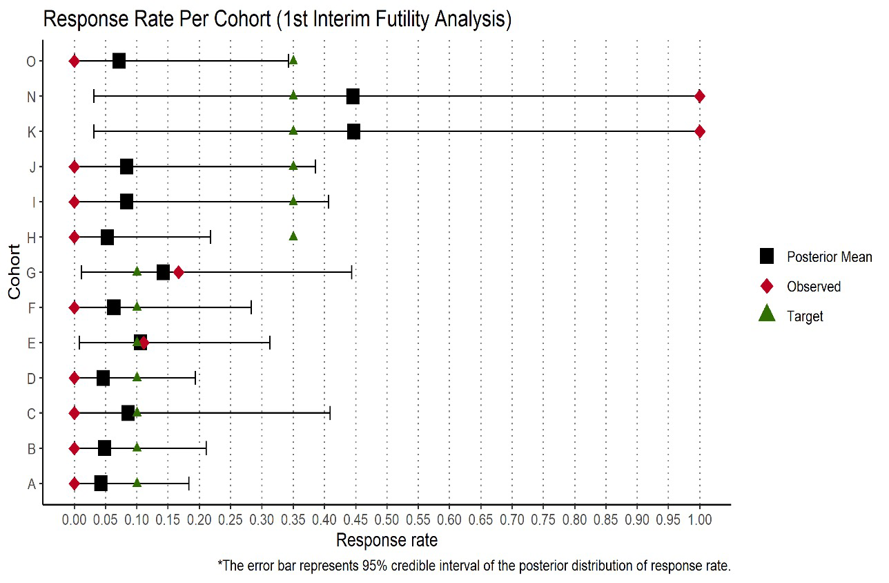
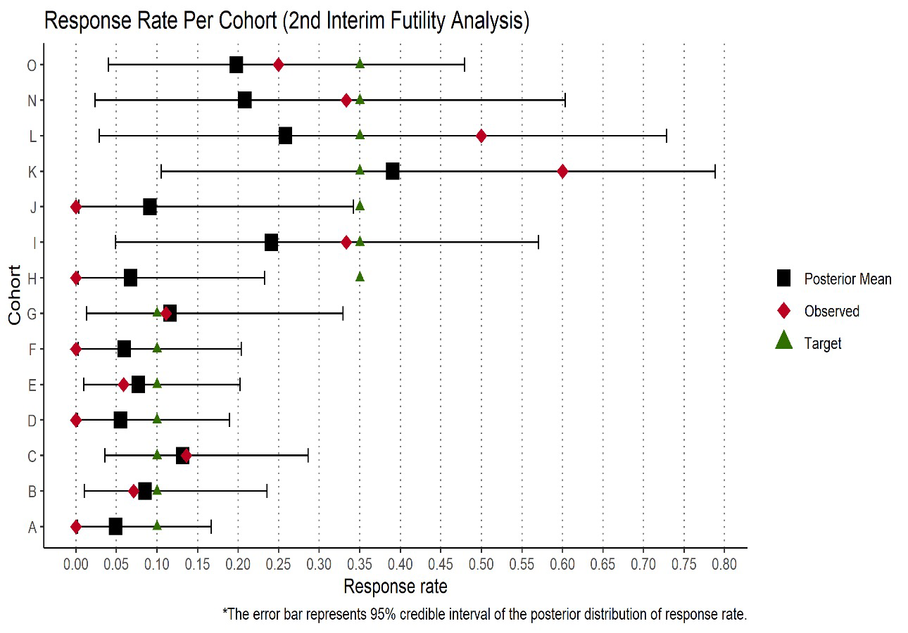
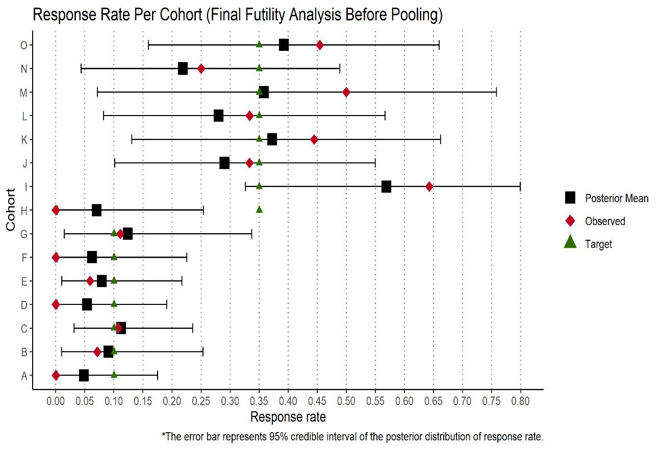
saveRDS(df_jandj,file="xxx.rds")

Perform operating characteristics analysis on the output datasets by running the script Analysis2.R.

Visualization of Futility Analysis

We selected a scenario half-half other 35 below to visualize the futility analysis using bayesian methods. The figures were generated in 1st IA, 2nd IA and final futility analysis before pooling.

The numbers below represents the target response rate for each cohort.

0.10 0.10 0.10 0.10 0.10 0.10 0.10 0.35 0.35 0.35 0.35 0.35 0.35 0.35 0.35

The sample code for the figures below is stored as PosteriorPlotExample.R.

1st Interim Futility Analysis

2nd Interim Futility Analysis

Final Futility Analysis Before Pooling

Main Code for BHM Simulation

function2.R

#######################################
## import library
#######################################
library(ggplot2)
library(dplyr)
library(tidyr)
library(gridExtra)
library(reshape)
library(invgamma)
library(bayesCT)
library(rjags)
library(tibble)
library(parallel)
library(doParallel)
library(rlist)

#######################################
## utility function
#######################################

summary_cohort <- function(data) {
  result <-
    data %>% group_by(tumor_group_assign) %>% summarise(n = n(), responders = sum(response))
  df <- as.data.frame(result)
  df <- df %>% mutate(prop=responders/n)
  return(df)
}

# function to remove key from a list
remove_from_list <- function(data,removelst){
  len <- length(removelst)
  texta <- "within(data, rm("
  textb <- "))"
  if (length(removelst) != 0){
    for (i in 1:len){
      data <- eval(parse(text=paste0(texta,removelst[i],textb)))
    }
  }
  return(data)
}

# update tumor prop weight
update_tumor_prop <- function(source,stopcohort){
  # source: source list
  # stopcohort: vec, the cohorts will be stopped
  prop_tumor_lst_2 <- remove_from_list(source,stopcohort)
  prop_tumor_lst_2 <- as.list(unlist(prop_tumor_lst_2)/sum(unlist(prop_tumor_lst_2)))
  return(prop_tumor_lst_2)
}

##############################################################################
# observed issues:
# 1. e.g. stop cohort B in IA1 due to low posterior prob, 
#    but high in IA2. How to decide? since IA is futility IA, I think it is
#    more reasonable to stop cohort B for all incoming recruitment.
#
##############################################################################

#######################################
## import functions
#######################################

trialsingle <- function(simindex,
                        IA,
                        accrate,
                        ss,
                        datacut,
                        multiplier,
                        tumorprop,
                        trueorr,
                        trdur,
                        cap,
                        norm_a=-2.19,
                        norm_b=4,
                        mean_tau=2,
                        weight_tau=0.75,
                        mcmc_seed=100,
                        mcmc_iter=5000,
                        futprob=0.25,
                        probfut=0.40,
                        minsub=5,
                        succprob=0.25,
                        probsucc=0.8,
                        p0=0.15,
                        alpha=0.05){
  # simindex: the index of sim trial
  # IA: indicate which stage of IA
  # accrate: float, accrual rate during the trial
  # ss: integer, total sample size in the whole trial
  # datacut: vec of integer, the total sample size in each IA, e.g. c(50,120,200)
  # tumorprop: list, the prevalence of tumor type
  # trueorr: list, the orr for binomial distribution
  # multiplier: float, give an upper limit for sample size, typically x1.5
  
  # detect the number of cores for parallel computing
  # n.cores <- detectCores()
  
  # #################
  # general setting
  # #################
  tumor_type_overall <- LETTERS[1:length(tumorprop)] # generate tumor type
  tumorprop.lst <- setNames(as.list(tumorprop),tumor_type_overall)
  tumororr.lst <- setNames(as.list(trueorr),tumor_type_overall)
  tumor.cap.index <- setNames(as.list(rep(NA,length(tumorprop))),tumor_type_overall) # locate where to stop recruitment due to cap
  ########################
  # simulate 1st interim
  ########################
  # generate simulated data which is larger than the sample size 
  n1sample <- multiplier*ss
  
  # initiate data container & generate random numbers
  simindex_vec <- rep(simindex,n1sample)
  id <- as.integer(seq(from=1,to=n1sample,by=1)) # subject id
  enroll_pattern <- enrollment(param = accrate, N_total = n1sample) # enroll pattern
  complete.tr <- enroll_pattern + trdur
  tumor_group_assign <- sample(tumor_type_overall, size = n1sample, replace = TRUE, prob = tumorprop)
  IA.flag <- rep(FALSE,n1sample)
  keep.flag <- rep(FALSE,n1sample) # indicate if this record is kept
  response <- rep(FALSE,n1sample) # indicate if this record is kept
  
  # data manipulate
  IA1.df <- data.frame(simindex_vec,
                       id,
                       enroll_pattern,
                       complete.tr, 
                       tumor_group_assign,
                       response,
                       IA.flag,
                       keep.flag)
  
  # initiate the sample size for IA1
  IA1.ss <- 0
  tumor.counter <- setNames(as.list(rep(0,length(tumorprop))),tumor_type_overall)
  stopflag <- FALSE
  
  for (i in 1:nrow(IA1.df)){
    # search tumor type
    i.tumor <- IA1.df[i,"tumor_group_assign"]
    
    # check if the tumor type exceeds the cap
    if (tumor.counter[[i.tumor]] <= cap-1){
      i.tumor.orr <- tumororr.lst[[i.tumor]]
      IA1.df[i,"response"] <- rbinom(1,1,i.tumor.orr)
      # indicate if this record go to IA 1
      if (IA1.ss <= (datacut[1]-1)){
        IA1.df[i,"IA.flag"] <- TRUE
        IA1.df[i,"keep.flag"] <- TRUE # whether records are kept in dataset
        IA1.maxtrassess <-  IA1.df[i,"complete.tr"]
      } else if ((IA1.ss > datacut[1]-1) & IA1.df[i,"enroll_pattern"] <= IA1.maxtrassess){
        IA1.df[i,"keep.flag"] <- TRUE
      } else {
        stopflag <- TRUE
      }
    } else {
      next
    }
    
    if (stopflag == FALSE) {
      # count the sample size for each tumor type
      tumor.counter[[i.tumor]] <- tumor.counter[[i.tumor]] +1
      # sum up to check the sample size
      IA1.ss <- sum(unlist(tumor.counter))
    } else {
      # record the final row index
      IA1.rowindex <- i
      break
    }
  }
  
  # output data
  IA1.df <- IA1.df %>%
    mutate(IA = ifelse(IA.flag==TRUE,
                       1,
                       ifelse(IA.flag==FALSE & keep.flag==TRUE,2,NA)))
  
  # a name list of no-go cohort due to CAP
  cap.nogo <- names(unlist(tumor.counter)[unlist(tumor.counter)>=cap])
  
  ###################################
  # Bayes IA 1 - futility analysis
  ###################################
  
  # set the parameter for normal
  a = norm_a
  b = norm_b
  
  # set the parameter for inverse gamma
  invg_a <- weight_tau / 2
  invg_b <- (mean_tau ^ 2) * weight_tau / 2
  
  # subset data for analysis
  adam <- IA1.df %>%
    filter(IA <= 1 & (!is.na(IA)))
  
  summary_adam <- summary_cohort(adam)
  
  # set burn in
  burn.in = 2000
  
  # DEFINE the BH model
  bayes_model <- "model{
    # Likelihood model for PiG
    for (i in 1:length(K)){
      K[i] ~ dbin(orr[i],n[i])
      orr[i] <- exp(thetag[i])/(1+exp(thetag[i]))
    }
    for (i in 1:length(K)){
      thetag[i] ~ dnorm(mu,tau2)
    }

    # Prior model for thetag,mu,tau2
    mu ~ dnorm(a, b)
    # sigma2 <- 1/tau2
    ## inverse gamma
    tau2 ~ dgamma(alpha,beta)
    }"
  
  bayes_jags_IA <- jags.model(
    textConnection(bayes_model),
    data = list(
      a = a,
      b = b,
      K = summary_adam$responders,
      alpha = invg_a,
      beta = invg_b,
      n = summary_adam$n
    ),
    inits = list(.RNG.name = "base::Wichmann-Hill", .RNG.seed = mcmc_seed),
    quiet = TRUE
  )
  # mcmc to generate the posterior
  update(bayes_jags_IA, burn.in)
  bayes_sim_IA <-
    coda.samples(model = bayes_jags_IA,
                 variable.names = c("orr"),
                 n.iter = mcmc_iter)
  # Store the chains in a matrix -- source of posterior of orr
  bayes_chains_IA <- bayes_sim_IA[[1]]
  colnames(bayes_chains_IA) <- summary_adam$tumor_group_assign
  # futility
  futility_decision_IA <-
    apply(bayes_chains_IA > futprob, MARGIN = 2, FUN = mean)
  ###  decide which cohort should be stopped due to posterior
  # bayesian stop due to futility: posterior < probfut and min subjects >= minsub
  stop_bayes_post1 <-
    intersect(summary_adam$tumor_group_assign[which(futility_decision_IA <
                                                      probfut)],
              (summary_adam %>% filter(n >= minsub))$tumor_group_assign)
  # overall: which cohorts should be stopped
  overall.stop <- union(cap.nogo, stop_bayes_post1)
  
  ########################
  # simulate 2nd interim
  ########################
  stopflag <- FALSE
  for (j in IA1.rowindex:nrow(IA1.df)){
    # search tumor type
    i.tumor <- IA1.df[j,"tumor_group_assign"]
    
    if (i.tumor %in% overall.stop){
      next
    }
    
    # check if the tumor type exceeds the cap
    if (tumor.counter[[i.tumor]] <= cap-1){
      i.tumor.orr <- tumororr.lst[[i.tumor]]
      IA1.df[j,"response"] <- rbinom(1,1,i.tumor.orr)
      # indicate if this record go to IA 1
      if (IA1.ss <= (datacut[2]-1)){
        IA1.df[j,"IA.flag"] <- TRUE
        IA1.df[j,"keep.flag"] <- TRUE # whether records are kept in dataset
        IA1.maxtrassess <-  IA1.df[j,"complete.tr"]
        IA1.df[j,"IA"] <- 2
      } else if ((IA1.ss > datacut[2]-1) & IA1.df[j,"enroll_pattern"] <= IA1.maxtrassess){
        IA1.df[j,"keep.flag"] <- TRUE
        IA1.df[j,"IA"] <- 3
      } else {
        stopflag <- TRUE
      }
    } else {
      next
    }
    
    if (stopflag == FALSE) {
      # count the sample size for each tumor type
      tumor.counter[[i.tumor]] <- tumor.counter[[i.tumor]] +1
      # sum up to check the sample size
      IA1.ss <- sum(unlist(tumor.counter))
    } else {
      # record the final row index
      IA2.rowindex <- j
      break
    }
  }
  
  # a name list of no-go cohort due to CAP
  cap.nogo <- names(unlist(tumor.counter)[unlist(tumor.counter)>=cap])
  
  ###################################
  # Bayes IA 2 - futility analysis
  ###################################
  
  # subset data for analysis
  adam <- IA1.df %>%
    filter(IA <= 2 & (!is.na(IA)))
  
  summary_adam <- summary_cohort(adam)
  
  # mcmc to generate the posterior
  bayes_jags_IA <- jags.model(
    textConnection(bayes_model),
    data = list(
      a = a,
      b = b,
      K = summary_adam$responders,
      alpha = invg_a,
      beta = invg_b,
      n = summary_adam$n
    ),
    inits = list(.RNG.name = "base::Wichmann-Hill", .RNG.seed = mcmc_seed),
    quiet = TRUE
  )
  update(bayes_jags_IA, burn.in)
  bayes_sim_IA <-
    coda.samples(model = bayes_jags_IA,
                 variable.names = c("orr"),
                 n.iter = mcmc_iter)
  # Store the chains in a matrix -- source of posterior of orr
  bayes_chains_IA <- bayes_sim_IA[[1]]
  colnames(bayes_chains_IA) <- summary_adam$tumor_group_assign
  # futility
  futility_decision_IA <-
    apply(bayes_chains_IA > futprob, MARGIN = 2, FUN = mean)
  ###  decide which cohort should be stopped due to posterior
  # bayesian stop due to futility: posterior < probfut and min subjects >= minsub
  stop_bayes_post2 <-
    intersect(summary_adam$tumor_group_assign[which(futility_decision_IA <
                                                      probfut)],
              (summary_adam %>% filter(n >= minsub))$tumor_group_assign)
  stop.bayes <- unique(union(stop_bayes_post1,stop_bayes_post2))
  # overall: which cohorts should be stopped
  overall.stop <- union(cap.nogo, stop.bayes)
  
  ########################
  # simulate finalinterim
  ########################
  stopflag <- FALSE
  for (m in IA2.rowindex:nrow(IA1.df)){
    # search tumor type
    i.tumor <- IA1.df[m,"tumor_group_assign"]
    
    if (i.tumor %in% overall.stop){
      next
    }
    
    # check if the tumor type exceeds the cap
    if (tumor.counter[[i.tumor]] <= cap-1){
      i.tumor.orr <- tumororr.lst[[i.tumor]]
      IA1.df[m,"response"] <- rbinom(1,1,i.tumor.orr)
      # indicate if this record go to IA 1
      if (IA1.ss <= (datacut[3]-1)){
        IA1.df[m,"IA.flag"] <- TRUE
        IA1.df[m,"keep.flag"] <- TRUE # whether records are kept in dataset
        IA1.maxtrassess <-  IA1.df[m,"complete.tr"]
        IA1.df[m,"IA"] <- 3
      } else {
        stopflag <- TRUE
      }
    } else {
      next
    }
    
    if (stopflag == FALSE) {
      # count the sample size for each tumor type
      tumor.counter[[i.tumor]] <- tumor.counter[[i.tumor]] +1
      # sum up to check the sample size
      IA1.ss <- sum(unlist(tumor.counter))
    } else {
      # record the final row index
      IA3.rowindex <- m
      break
    }
  }
  
  ###################################
  # Bayes Final 
  ###################################
  
  # subset data for analysis
  adam <- IA1.df %>%
    filter(IA <= 3 & (!is.na(IA)))
  
  summary_adam <- summary_cohort(adam)
  
  # mcmc to generate the posterior
  bayes_jags_IA <- jags.model(
    textConnection(bayes_model),
    data = list(
      a = a,
      b = b,
      K = summary_adam$responders,
      alpha = invg_a,
      beta = invg_b,
      n = summary_adam$n
    ),
    inits = list(.RNG.name = "base::Wichmann-Hill", .RNG.seed = mcmc_seed),
    quiet = TRUE
  )
  update(bayes_jags_IA, burn.in)
  bayes_sim_IA <-
    coda.samples(model = bayes_jags_IA,
                 variable.names = c("orr"),
                 n.iter = mcmc_iter)
  # Store the chains in a matrix -- source of posterior of orr
  bayes_chains_IA <- bayes_sim_IA[[1]]
  colnames(bayes_chains_IA) <- summary_adam$tumor_group_assign
  
  ###################################
  # Bayes Final - futility analysis
  ###################################
  
  # futility
  futility_decision_IA <-
    apply(bayes_chains_IA > futprob, MARGIN = 2, FUN = mean)
  ###  decide which cohort should be stopped due to posterior
  # bayesian stop due to futility: posterior < probfut and min subjects >= minsub
  stop_bayes_post3 <-
    intersect(summary_adam$tumor_group_assign[which(futility_decision_IA <
                                                      probfut)],
              (summary_adam %>% filter(n >= minsub))$tumor_group_assign)
  stop.bayes <- unique(union(stop.bayes,stop_bayes_post3)) # will not pool
  
  ############################################
  # Bayes Final - Bayesian efficacy analysis
  ############################################
  ## single cohort success
  by_cohort_decision_FA <- apply(bayes_chains_IA>succprob,MARGIN = 2,FUN=mean)
  single_cohort_succ <- summary_adam$tumor_group_assign[which(by_cohort_decision_FA>probsucc)]
  single_success <- ifelse(length(single_cohort_succ)>0,TRUE,FALSE)
  
  ## get FWER
  nonactive <- names(tumororr.lst[tumororr.lst<=0.15]) # get the non-active histology
  if (length(single_cohort_succ)>0){
    if(sum(is.element(single_cohort_succ,nonactive))>=1){
      fwerflag <- TRUE
    } else {
      fwerflag <- FALSE
    }
  } else {
    fwerflag <- FALSE
  }
  
  ## overall success by pooling via exact binomial test: H0 p<=p0, H1 p>p0
  pooldat <- summary_adam %>% filter(!tumor_group_assign %in% stop.bayes)
  pooltotalresp <- sum(pooldat$responders)
  poolsamplesize <- sum(pooldat$n)
  poolresprate <- round(pooltotalresp/poolsamplesize,3)
  if (poolsamplesize>0){
    poolingtest <- ifelse(as.numeric(binom.test(x=pooltotalresp,n=poolsamplesize,p=p0,alternative = "greater")$p.value <= (alpha) ),TRUE,FALSE)
  } else {
    poolingtest <- FALSE
  }
  overalltotalresp <- sum(summary_adam$responders)
  overallsamplesize <- sum(summary_adam$n)
  overallresprate <- round(overalltotalresp/overallsamplesize,3)
  
  # FPR for pooled analysis
  # re-calculate tumor proportion (normalizing the weight)
  not_appear_insim <- names(remove_from_list(data=tumorprop.lst,removelst = summary_adam$tumor_group_assign))
  stop_cohort <- unique(union(not_appear_insim,stop.bayes))
  norm_tumorprop_weight <- update_tumor_prop(source=tumorprop.lst,stopcohort=stop_cohort)
  ## initial the flag for mixing non-active
  mixnonactflag <- FALSE
  if (poolsamplesize != 0){
    norm_tumorprop_weight.df <- data.frame(norm_tumorprop_weight) 
    # pooldat.subset <- pooldat[,c("tumor_group_assign","prop")]
    # pooldat.subset2 <- pooldat.subset %>%
    #   pivot_wider(names_from = tumor_group_assign, values_from = prop) %>%
    #   as.data.frame()
    pooldat.subset2 <- data.frame(remove_from_list(data = tumororr.lst,removelst = stop_cohort))
    mixnonactflag <- ifelse(sum(pooldat.subset2[1,]<=0.15)>=1 & poolingtest == TRUE,TRUE,FALSE)
    poolorr <- rbind(norm_tumorprop_weight.df,pooldat.subset2)
    weighted.orr <- sum(poolorr[1,]*poolorr[2,])
    if (poolingtest == TRUE & (weighted.orr-0.15)<=1e-3){
      fprflag <- TRUE
    } else {
      fprflag <- FALSE
    } 
  } else {
    fprflag <- FALSE
  }
  
  # record those cohorts enter pooling analysis
  tumor.futstop <- setNames(as.list(rep(0,length(tumor_type_overall))),tumor_type_overall)
  for (item in stop.bayes){
    tumor.futstop[[item]] <- tumor.futstop[[item]]+1
  }
  
  # duration 
  maxdur <- max(adam$enroll_pattern)
  
  # efficacy FA output
  index <- min(adam$simindex_vec)
  df0 <- data.frame(index = index)
  df1 <- t(as.data.frame(by_cohort_decision_FA>probsucc))
  rownames(df1) <- c()   
  df2 <- data.frame(singlesucc = single_success,
                    poolsucc = poolingtest,
                    pooltotalresp = pooltotalresp,
                    poolsamplesize = poolsamplesize,
                    poolresprate = poolresprate,
                    overalltotalresp = overalltotalresp,
                    overallsamplesize = overallsamplesize,
                    overallresprate = overallresprate,
                    maxdur = maxdur,
                    fwer = fwerflag,
                    fpr = fprflag,
                    mixnonact = mixnonactflag)
  df3 <- as.data.frame(tumor.futstop)
  colnames(df3) <- paste0(colnames(df3),"_pool")
  df <- cbind(df0,df1,df2,df3)
  
  return(df)
}

TrialSim2.R

#####
#run
#####

source("functions2.R")

## TEST code
simindex = 1
tumorprop = c(18,18,13,13,10,5,4,4,3,2,2,1,1,1,5)*0.01
# trueorr = rep(0.15,15)
# trueorr = rep(0.25,15)
# trueorr = rep(0.35,15)
# trueorr = c(rep(0.10,7),rep(0.35,7),0.15) # use half-half other 15 settings
 trueorr = c(rep(0.10,7),rep(0.35,8)) # use half-half other 35 settings
# trueorr = c(rep(0.10,2),rep(0.15,3),0.35,rep(0.15,9)) # use Cholangio35 settings
p.target = 0.15
IA = 1
accrate = 10/7
ss = 200
datacut = c(60,130,200) # 200 is final analysis
multiplier = 3
trdur = 4*7
cap = 30

## parallel

set.seed(123)

iter = 5000

myCluster <- makeCluster(10)
registerDoParallel(myCluster)

df_jandj = foreach(it=1:iter,.combine=dplyr::bind_rows)%dopar%{
  source("functions2.R")
  trialsingle(simindex,
              IA,
              accrate,
              ss,
              datacut,
              multiplier,
              tumorprop,
              trueorr,
              trdur,
              cap,
              norm_a=-2.19,
              norm_b=1/4,
              mean_tau=2,
              weight_tau=0.75,
              mcmc_seed=100,
              mcmc_iter=5000,
              futprob=0.25,
              probfut=0.40,
              minsub=5,
              succprob=0.25,
              probsucc=0.8,
              p0=0.15,
              alpha=0.05)
}

stopCluster(myCluster)

saveRDS(df_jandj,file="df_halfhalf35.rds")

Analysis2.R

#######################################
## analysis the result
#######################################
library(ggplot2)
library(rtables)

folder = "xxxx" # Set target working dir

# Start writing to an output file
df_all15 <- readRDS(file=paste0(folder,"df_all15.rds"))
df_all25 <- readRDS(file=paste0(folder,"df_all25.rds"))
df_all35 <- readRDS(file=paste0(folder,"df_all35.rds"))
df_halfhalf35 <- readRDS(file=paste0(folder,"df_halfhalf35.rds"))
df_halfhalf15 <- readRDS(file=paste0(folder,"df_halfhalf15.rds"))
df_Cholangio35 <- readRDS(file=paste0(folder,"df_Cholangio35.rds"))

write2txt <- function(name,data,file,append=FALSE){
  # cohort vec
  trueorr = c(rep(0.15,7),rep(0.35,8)) # use half-half other 35 settings
  cohort_vec <- LETTERS[1:length(trueorr)]
  cohort_vec_pool <- paste0(cohort_vec,"_pool")
  
  if (append==FALSE){
    
    sink(file)
    
    cat(name,"\n", "-----------------","\n")
    
    # single success
    df1 <- data[,c(cohort_vec,"singlesucc")]
    df1[is.na(df1)] <- 0
    singlesucc.df <- as.data.frame(apply(df1,MARGIN = 2, mean))
    print(singlesucc.df[1:(nrow(singlesucc.df)-1),,drop=FALSE])
    cat(">> Ppn of success: ", singlesucc.df[nrow(singlesucc.df),1],"\n")
    
    # overall success (by exact binom test)
    # hypothesis test: h1: p>p0=0.35
    cat(">> Power: ",mean(data[,c("poolsucc")]),"\n")
    
    # fwer for single success
    cat(">> FWER: ",mean(data[,c("fwer")]),"\n")
    
    # fpr for pool
    cat(">> FPR: ",mean(data[,c("fpr")]),"\n")
    
    # mixing non-active
    cat(">> Mixing non-active: ",mean(data[,c("mixnonact")]),"\n")
    
    # mean duration
    cat(">> mean duration (days): ",mean(data[,c("maxdur")]),"\n")
    sink() 
  } else {
    sink(file,append = TRUE)
    
    cat("\n",name,"\n", "-----------------","\n")
    
    # single success
    df1 <- data[,c(cohort_vec,"singlesucc")]
    df1[is.na(df1)] <- 0
    singlesucc.df <- as.data.frame(apply(df1,MARGIN = 2, mean))
    print(singlesucc.df[1:(nrow(singlesucc.df)-1),,drop=FALSE])
    cat(">> Ppn of success: ", singlesucc.df[nrow(singlesucc.df),1],"\n")
    
    # overall success (by exact binom test)
    # hypothesis test: h1: p>p0=0.35
    cat(">> Power: ",mean(data[,c("poolsucc")]),"\n")
    
    # fwer for single success
    cat(">> FWER: ",mean(data[,c("fwer")]),"\n")
    
    # fpr for pool
    cat(">> FPR: ",mean(data[,c("fpr")]),"\n")
    
    # mixing non-active
    cat(">> Mixing non-active: ",mean(data[,c("mixnonact")]),"\n")
    
    # mean duration
    cat(">> mean duration (days): ",mean(data[,c("maxdur")]),"\n")
    sink()
  }
}

folder = "xxxx" # Set target working dir
write2txt(name="df_all15",data=df_all15,file = paste0(folder,"allscen.txt"))
write2txt(name="df_all35",data=df_all35,file = paste0(folder,"allscen.txt"),append = TRUE)
write2txt(name="df_all25",data=df_all25,file = paste0(folder,"allscen.txt"),append = TRUE)
write2txt(name="df_halfhalf35",data=df_halfhalf35,file = paste0(folder,"allscen.txt"),append = TRUE)
write2txt(name="df_halfhalf15",data=df_halfhalf15,file = paste0(folder,"allscen.txt"),append = TRUE)
write2txt(name="df_Cholangio35",data=df_Cholangio35,file = paste0(folder,"allscen.txt"),append = TRUE)


# selection power plot
df2 <- df_jandj[cohort_vec_pool]
selection_power1 <- length(cohort_vec_pool)-apply(df2,MARGIN = 1,sum)
selection_power1_df <- as.data.frame(table(selection_power1))
selection_power1_df <- selection_power1_df %>%
  mutate(type=paste0(">=",as.character(selection_power1)),sum=0)
for (rowi in 1:nrow(selection_power1_df)){
  selection_power1_df[rowi,"sum"] <- sum(selection_power1_df$Freq[rowi:nrow(selection_power1_df)])
}
selection_power1_df <- selection_power1_df %>%
  mutate(perc=sum/nrow(df_jandj))
p <- ggplot(data=selection_power1_df,aes(x=type,y=perc)) +
  geom_bar(stat = "identity",width=0.2) +
  scale_x_discrete(limits=selection_power1_df$type) +
  geom_text(aes(label = perc), vjust = -0.3) +
  theme_bw()
p



###########################
## without cPR/cCR
###########################

df_all25_noconfirm <- readRDS(file="df_all25_noconfirm.rds")
write2txt(name="df_all25_noconfirm",data=df_all25_noconfirm,file = paste0(folder,"df_all25_noconfirm.txt"))


###############################################
## all 25 and futility stop prob = 0.34
###############################################

df_all25_probfut34 <- readRDS(file="df_all25_probfut34.rds")
write2txt(name="df_all25_probfut34",data=df_all25_probfut34,file = paste0(folder,"df_all25_probfut34.txt"))

###############################################
## all 25 and futility stop prob = 0.30
###############################################

df_all25_probfut30 <- readRDS(file="df_all25_probfut30.rds")
write2txt(name="df_all25_probfut30",data=df_all25_probfut30,file = paste0(folder,"df_all25_probfut30.txt"))